Chapter 5 Assessment of the nature of batch effects

5.1 Simulations

5.1.1 Mean = 5, and unequal variance

‘Systematic’ refers to homogeneous change amongst all microbial variables (OTUs) due to having the same source of variation. We illustrate this concept in a linear model framework where batch and treatment regression coefficients are estimated simultaneously on each OTU. For a given batch effect and a given OTU, we can formulate the systematic assumption as:

\[\beta_{j} \sim N(\mu,\sigma^{2})\]

where \(\beta_{j}\) is the batch regression coefficient of OTU\(_{j}\) (\(j = 1,...,p\)). Here we consider the simplest case of a linear model with one batch predictor, but this formulation could be extended to a model with multiple batch predictors where the batch regression coefficients can represent more than two batch levels. In a univariate model that tests each OTU individually, then the distribution of the batch coefficients of all OTUs is Gaussian with a mean \(\mu\), and standard deviation \(\sigma\). This indicates that the batch effect has a similar, though not necessarily identical, influence on all OTUs.

To illustrate the type of batch effects, we simulated a set of data with 50 samples and 10,000 OTUs each, based on the simulation approach from (Gagnon-Bartsch, Jacob, and Speed 2013).

The dataset with a systematic batch effect:

• \(\beta_{j} \sim N(5,1^{2})\) for \(j=1,...,p\) OTUs;
  
• \(\sigma_{j} \sim N(0,2^{2})\) for \(j=1,...,p\) OTUs; This variance per OTU is aimed to simulate data as realistically as possible.
  
• \(\beta_{ij} \sim N(\beta_{j}, \sigma_{j}^{2})\) for \(i = 1,...,n\) samples.

# Create the simulated data
m <- 50
n <- 10000
nc <- 1000 # negative controls without treatment effects
p <- 1
k <- 1
ctl <- rep(FALSE, n)
ctl[1:nc] <- TRUE
# treatment effect
X <- matrix(c(rep(0, floor(m/2)), rep(1, ceiling(m/2))), m, p)
beta <- matrix(rnorm(p*n, 5, 1), p, n) #treatment coefficients
beta[ ,ctl] <- 0
# batch effect
W <- as.matrix(rep(0, m), m, k)
W[c(1:12,38:50), 1] <-  1
alpha <- matrix(rnorm(k*n, 5, 1), k, n)
Y_alpha <- sapply(alpha, function(alpha){rnorm(m, mean =  alpha, 
                                              abs(rnorm(1, mean = 0, sd = 2)))})
YY_alpha <- apply(Y_alpha, 2, function(x){x*W})

epsilon <- matrix(rnorm(m*n, 0, 1), m, n)
Y <- X%*%beta + YY_alpha + epsilon


# estimate batch coefficient for each OTU
w.cof <- c()
for(i in 1:ncol(Y)){
  res <- lm(Y[ ,i] ~ X + W)
  sum.res <- summary(res)
  w.cof[i] <- sum.res$coefficients[3,1]
}

par(mfrow = c(2,2))
hist(w.cof,col = 'gray')
plot(density(w.cof))
qqnorm(w.cof)
qqline(w.cof, col = 'red')
par(mfrow = c(1,1))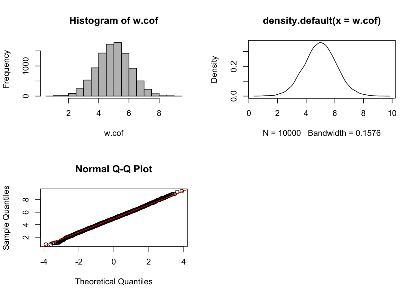

The histogram, density plot and quantile–quantile plot are plotted using estimated batch regression coefficients \(\hat{\beta}_{j}\) for each OTU \(j\). These plots display the distribution of batch coefficients is very close to normal, indicating a systematic batch effect.

5.1.2 Mean = 0 or 5, and unequal variance

Non-systematic batch effects have a heterogeneous influence on microbial variables. Using a linear model framework, as described previously, we can formulate this non-systematic assumption as:

\[ \beta'_{j} \sim \begin{cases} N(0,\delta^{2}) & \text{for OTUs with no batch effect,} \\ N(\mu,\sigma^{2}) & \text{for OTUs with batch effect.} \end{cases} \]

Therefore, the batch regression coefficients \(\beta'_{j}\) may follow skewed distributions with several modes.

The dataset with non-systematic batch effect:

• \(\beta'_{t} \sim N(0,1^{2})\) and \(\beta'_{k} \sim N(5,1^{2})\) for \(t=1,...,T\) OTUs, \(k=1,...,K\) OTUs and \(T=\frac{3}{4}p\), \(K=\frac{1}{4}p\);
  
• \(\sigma'_{j} \sim N(0,2^{2})\) for \(j=1,...,p\) OTUs;
  
• \(\beta'_{ij} \sim N(\beta'_{j}, \sigma_{j}^{'2})\) for \(i = 1,...,n\) samples.

# Create the simulated data
m <- 50
n <- 10000
nc <- 1000 # negative controls without treatment effects
p <- 1
k <- 1
ctl <- rep(FALSE, n)
ctl[1:nc] <- TRUE
# treatment effect
X <- matrix(c(rep(0, floor(m/2)), rep(1, ceiling(m/2))), m, p)
beta <- matrix(rnorm(p*n, 5, 1), p, n) #treatment coefficients
beta[ ,ctl] <- 0
# batch effect
W <- as.matrix(rep(0, m), m, k)
W[c(1:12,38:50), 1] <-  1
alpha2 <- matrix(sample(c(rnorm(k*(3*n/4), 0, 1),rnorm(k*(n/4), 5, 1)), n), k, n)
Y_alpha2 <- sapply(alpha2, function(alpha){rnorm(m, mean =  alpha, 
                                                sd = abs(rnorm(1, mean = 0, sd = 2)))})
YY_alpha2 <- apply(Y_alpha2, 2, function(x){x*W})

epsilon <- matrix(rnorm(m*n, 0, 1), m, n)
Y2 <- X%*%beta + YY_alpha2 + epsilon




w.cof2 <- c()
for(i in 1:ncol(Y2)){
  res <- lm(Y2[ ,i] ~ X + W)
  sum.res <- summary(res)
  w.cof2[i] <- sum.res$coefficients[3,1]
}

par(mfrow = c(2,2))
hist(w.cof2, col = 'gray')
plot(density(w.cof2))
qqnorm(w.cof2)
qqline(w.cof2, col = 'red')
par(mfrow = c(1,1))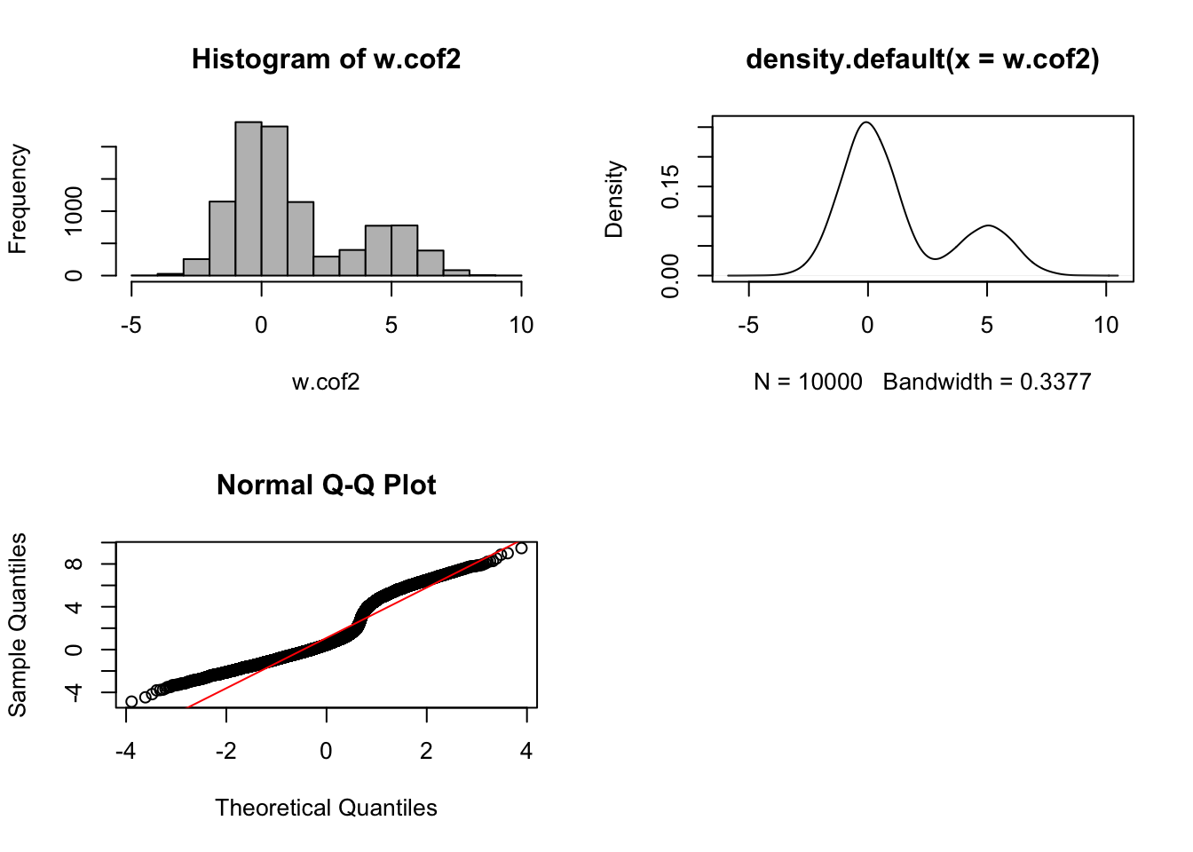

The histogram, density plot and quantile–quantile plot are plotted using estimated batch regression coefficients \(\hat{\beta}_{j}\) for each OTU \(j\), showing a bi-modal distribution. This distribution indicates a non-systematic batch effect.

We observed similar patterns in our real case studies, suggesting that the batch effects are mixed with multiple sources and are non-systematic (see the examples below).

5.2 Real data

We also estimate the batch regression coefficients for each OTU in real datasets to assess the nature of batch effects.

5.2.1 Sponge data

sponge.b.coeff <- c()
for(i in 1:ncol(sponge.tss.clr)){
  res <- lm(sponge.tss.clr[ ,i] ~ sponge.trt + sponge.batch)
  sum.res <- summary(res)
  sponge.b.coeff[i] <- sum.res$coefficients[3,1]
}

par(mfrow = c(2,2))
hist(sponge.b.coeff,col = 'gray')
plot(density(sponge.b.coeff))
qqnorm(sponge.b.coeff)
qqline(sponge.b.coeff, col='red')
par(mfrow = c(1,1))

In sponge data, the histogram, density plot and quantile–quantile plot are also plotted using estimated batch regression coefficients \(\hat{\beta}_{j}\) for each OTU \(j\). The bi-modal distribution indicates a non-systematic batch effect, which is similar as the results from simulation with non-systematic batch effects.

5.2.2 AD data

ad.b.coeff <- c()
ad.batch.relevel <- relevel(ad.batch, '01/07/2016')
for(i in 1:ncol(ad.clr)){
  res <- lm(ad.clr[,i] ~ ad.trt + ad.batch.relevel)
  sum.res <- summary(res)
  ad.b.coeff[i] <- sum.res$coefficients[4,1]
}

par(mfrow = c(2,2))
hist(ad.b.coeff,col = 'gray')
plot(density(ad.b.coeff))
qqnorm(ad.b.coeff)
qqline(ad.b.coeff, col='red')
par(mfrow = c(1,1))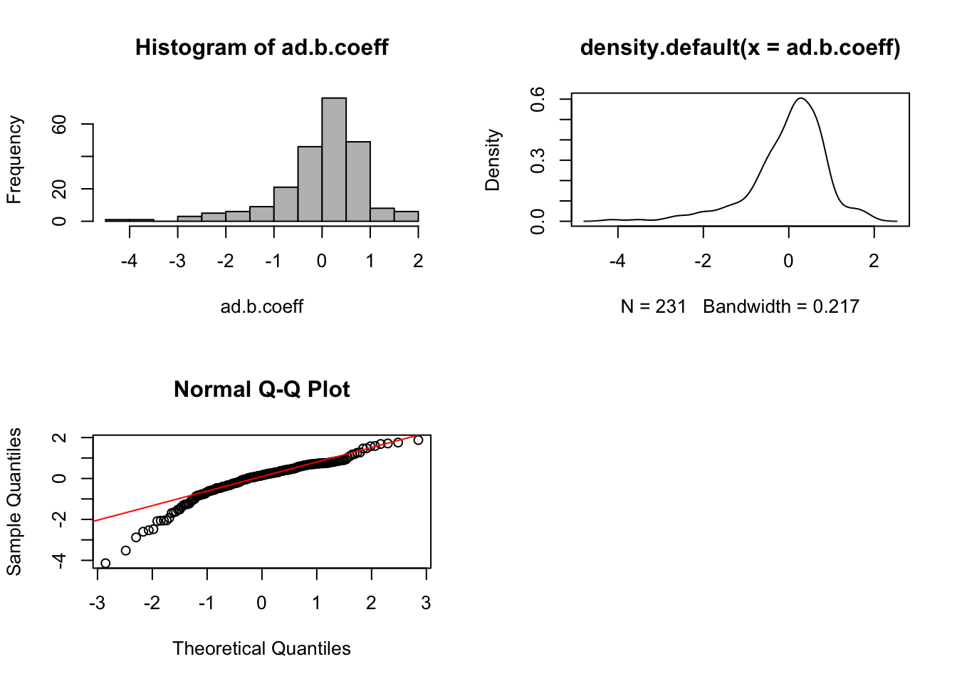

We observe similar results in AD data. The distribution of estimated batch regression coefficients is not normal. The batch effects therefore are non-systematic.

Bibliography

Gagnon-Bartsch, Johann A, Laurent Jacob, and Terence P Speed. 2013. “Removing Unwanted Variation from High Dimensional Data with Negative Controls.” Berkeley: Tech Reports from Dep Stat Univ California. Citeseer, 1–112.