Chapter 4 Methods evaluation
After batch effect adjustment, it is essential to evaluate its effectiveness. For simplicity, we focus only on strategies to assess batch effect correction methods, as methods that account for the batch effect often imply it has been assessed internally in the statistical model.
4.1 Diagnostic plots
Diagnostic plots are useful to visually evaluate for post-correction batch effects, as presented earlier in section ‘batch effect detection’.
4.1.1 Principal component analysis (PCA) with density plot per component
We apply PCA on both sponge and AD data before and after correction with different methods.
# sponge data
sponge.pca.before <- pca(sponge.tss.clr, ncomp = 3)
sponge.pca.bmc <- pca(sponge.bmc, ncomp = 3)
sponge.pca.combat <- pca(sponge.combat, ncomp = 3)
sponge.pca.limma <- pca(sponge.limma, ncomp = 3)
sponge.pca.percentile <- pca(sponge.percentile, ncomp = 3)
sponge.pca.svd <- pca(sponge.svd, ncomp = 3)

# ad data
ad.pca.before <- pca(ad.clr, ncomp = 3)
ad.pca.bmc <- pca(ad.bmc, ncomp = 3)
ad.pca.combat <- pca(ad.combat, ncomp = 3)
ad.pca.limma <- pca(ad.limma, ncomp = 3)
ad.pca.percentile <- pca(ad.percentile, ncomp = 3)
ad.pca.svd <- pca(ad.svd, ncomp = 3)
ad.pca.ruv <- pca(ad.ruvIII, ncomp = 3)
We then plot these PCA sample plots with denisty plots per PC.
Note: BMC: batch mean centering; PN: percentile normalisation; rBE: removeBatchEffect; SVD: singular value decomposition
grid.arrange(sponge.pca.plot.before, sponge.pca.plot.bmc,
             sponge.pca.plot.combat, sponge.pca.plot.limma, ncol = 2)
grid.arrange(sponge.pca.plot.before, sponge.pca.plot.percentile,
             sponge.pca.plot.svd, ncol = 2)
In sponge data, SVD performed the worse, compared to BMC, removeBatchEffect and percentile normalisation, as it did not remove batch effects but removed tissue variation instead.
grid.arrange(ad.pca.plot.before, ad.pca.plot.bmc,
             ad.pca.plot.combat, ad.pca.plot.limma, ncol = 2)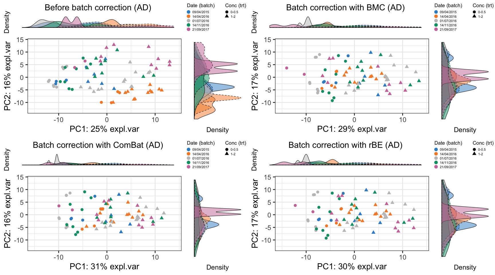
grid.arrange(ad.pca.plot.before, ad.pca.plot.percentile,
             ad.pca.plot.svd, ad.pca.plot.ruv, ncol = 2)
In AD data, BMC, removeBatchEffect, percentile normalisation and RUVIII removed the batch effects, and maintained the treatment effects. SVD did not removed the batch effect but decreased the treatment effects.
4.1.2 Density plot and box plot
# sponge data
sponge.before.df <- data.frame(value = sponge.tss.clr[ ,9], batch = sponge.batch)
sponge.boxplot.before <- box_plot_fun(data = sponge.before.df,
                                      x = sponge.before.df$batch,
                                      y = sponge.before.df$value,
                                      title = 'OTU9 - before (Sponge)',
                                      batch.legend.title = 'Gel (batch)')

sponge.bmc.df <- data.frame(value = sponge.bmc[ ,9], batch = sponge.batch)
sponge.boxplot.bmc <- box_plot_fun(data = sponge.bmc.df,
                                   x = sponge.bmc.df$batch,
                                   y = sponge.bmc.df$value,
                                   title = 'OTU9 - BMC (Sponge)',
                                   batch.legend.title = 'Gel (batch)')


sponge.combat.df <- data.frame(value = sponge.combat[ ,9], batch = sponge.batch)
sponge.boxplot.combat <- box_plot_fun(data = sponge.combat.df,
                                      x = sponge.combat.df$batch,
                                      y = sponge.combat.df$value,
                                      title = 'OTU9 - ComBat (Sponge)',
                                      batch.legend.title = 'Gel (batch)')


sponge.limma.df <- data.frame(value = sponge.limma[ ,9], batch = sponge.batch)
sponge.boxplot.limma <- box_plot_fun(data = sponge.limma.df,
                                     x = sponge.limma.df$batch,
                                     y = sponge.limma.df$value,
                                     title = 'OTU9 - rBE(Sponge)',
                                     batch.legend.title = 'Gel (batch)')

sponge.percentile.df <- data.frame(value = sponge.percentile[ ,9], batch = sponge.batch)
sponge.boxplot.percentile <- box_plot_fun(data = sponge.percentile.df,
                                          x = sponge.percentile.df$batch,
                                          y = sponge.percentile.df$value,
                                          title = 'OTU9 - PN (Sponge)',
                                          batch.legend.title = 'Gel (batch)')

sponge.svd.df <- data.frame(value = sponge.svd[ ,9], batch = sponge.batch)
sponge.boxplot.svd <- box_plot_fun(data = sponge.svd.df,
                                   x = sponge.svd.df$batch,
                                   y = sponge.svd.df$value,
                                   title = 'OTU9 - SVD (Sponge)',
batch.legend.title = 'Gel (batch)')grid.arrange(sponge.boxplot.before, sponge.boxplot.bmc,
sponge.boxplot.combat, sponge.boxplot.limma, ncol = 2)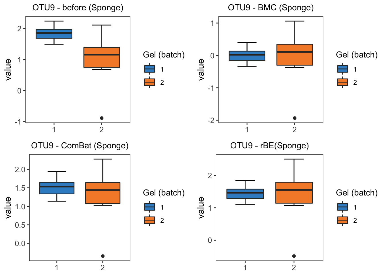
grid.arrange(sponge.boxplot.before, sponge.boxplot.percentile,
             sponge.boxplot.svd, ncol = 2)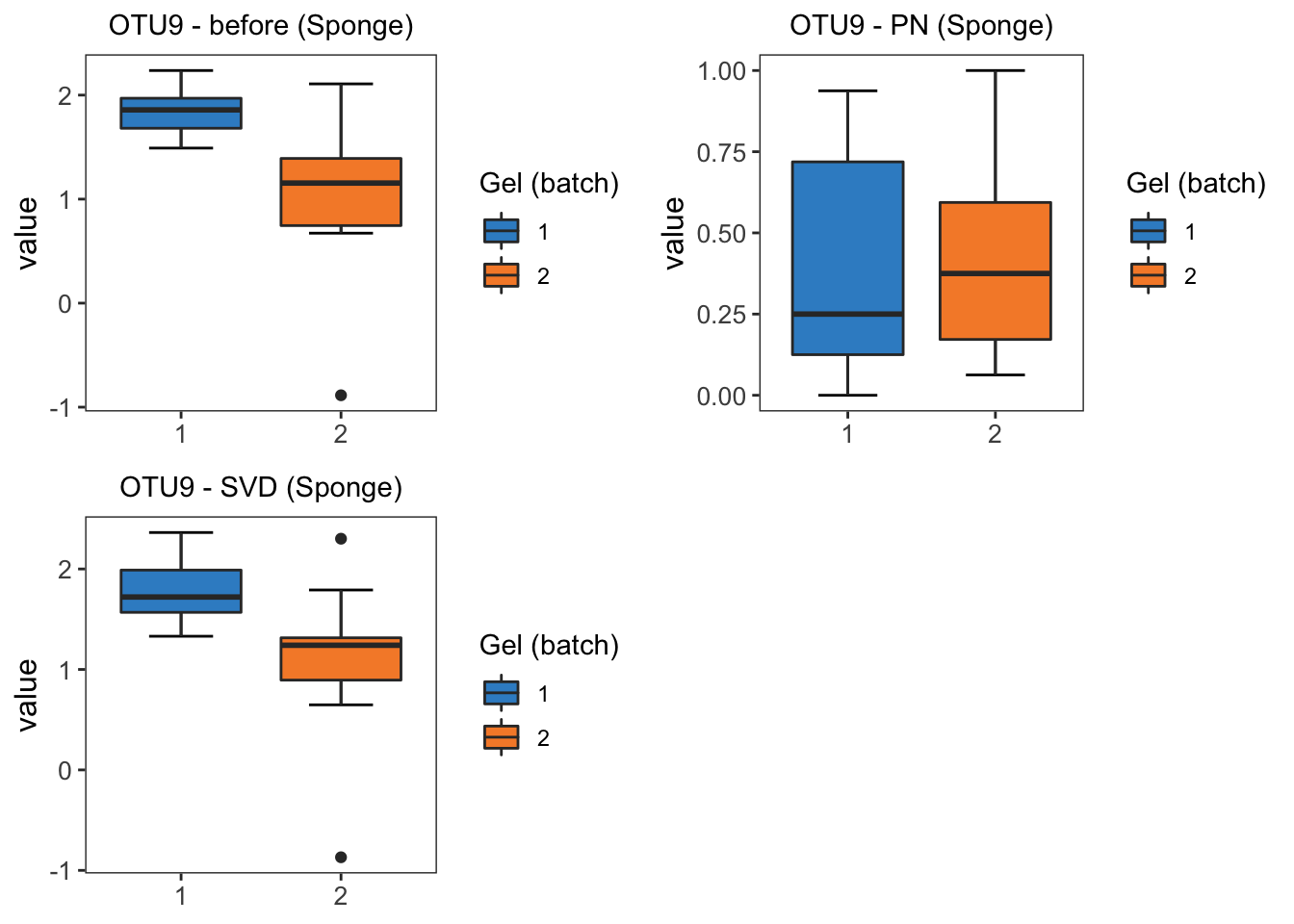
From the boxplots of OTU9 in sponge data, the difference between two batches are removed by BMC, ComBat, removeBatchEffect and percentile normalisation correction. Among these methods, percentile normalisation does not remove as much batch difference as the other methods.
# density plot
# before
sponge.dens.before <- ggplot(sponge.before.df, aes(x = value, fill = batch)) +
  geom_density(alpha = 0.5) + scale_fill_manual(values = color.mixo(1:10)) +
  labs(title = 'OTU9 - before (Sponge)', x = 'Value', fill = 'Gel (batch)') +
  theme_bw() + theme(plot.title = element_text(hjust = 0.5),
                     panel.grid = element_blank())

# BMC
sponge.dens.bmc <- ggplot(sponge.bmc.df, aes(x = value, fill = batch)) +
  geom_density(alpha = 0.5) + scale_fill_manual(values = color.mixo(1:10)) +
  labs(title = 'OTU9 - BMC (Sponge)', x = 'Value', fill = 'Gel (batch)') +
  theme_bw() + theme(plot.title = element_text(hjust = 0.5),
                     panel.grid = element_blank())


# ComBat
sponge.dens.combat <- ggplot(sponge.combat.df, aes(x = value, fill = batch)) +
  geom_density(alpha = 0.5) + scale_fill_manual(values = color.mixo(1:10)) +
  labs(title = 'OTU9 - ComBat (Sponge)', x = 'Value', fill = 'Gel (batch)') +
  theme_bw() + theme(plot.title = element_text(hjust = 0.5),
                     panel.grid = element_blank())


# removeBatchEffect
sponge.dens.limma <- ggplot(sponge.limma.df, aes(x = value, fill = batch)) +
  geom_density(alpha = 0.5) + scale_fill_manual(values = color.mixo(1:10)) +
  labs(title = 'OTU9 - rBE (Sponge)', x = 'Value', fill = 'Gel (batch)') +
  theme_bw() + theme(plot.title = element_text(hjust = 0.5),
                     panel.grid = element_blank())


# percentile normal
sponge.dens.percentile <- ggplot(sponge.percentile.df, aes(x = value, fill = batch)) +
  geom_density(alpha = 0.5) + scale_fill_manual(values = color.mixo(1:10)) +
  labs(title = 'OTU9 - PN (Sponge)', x = 'Value', fill = 'Gel (batch)') +
  theme_bw() + theme(plot.title = element_text(hjust = 0.5),
                     panel.grid = element_blank())


# SVD
sponge.dens.svd <- ggplot(sponge.svd.df, aes(x = value, fill = batch)) +
  geom_density(alpha = 0.5) + scale_fill_manual(values = color.mixo(1:10)) +
  labs(title = 'OTU9 - SVD (Sponge)', x = 'Value', fill = 'Gel (batch)') +
  theme_bw() + theme(plot.title = element_text(hjust = 0.5),
panel.grid = element_blank())grid.arrange(sponge.dens.before, sponge.dens.bmc,
sponge.dens.combat, sponge.dens.limma, ncol = 2)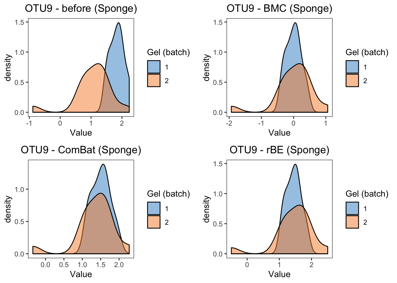
grid.arrange(sponge.dens.before, sponge.dens.percentile,
             sponge.dens.svd, ncol = 2)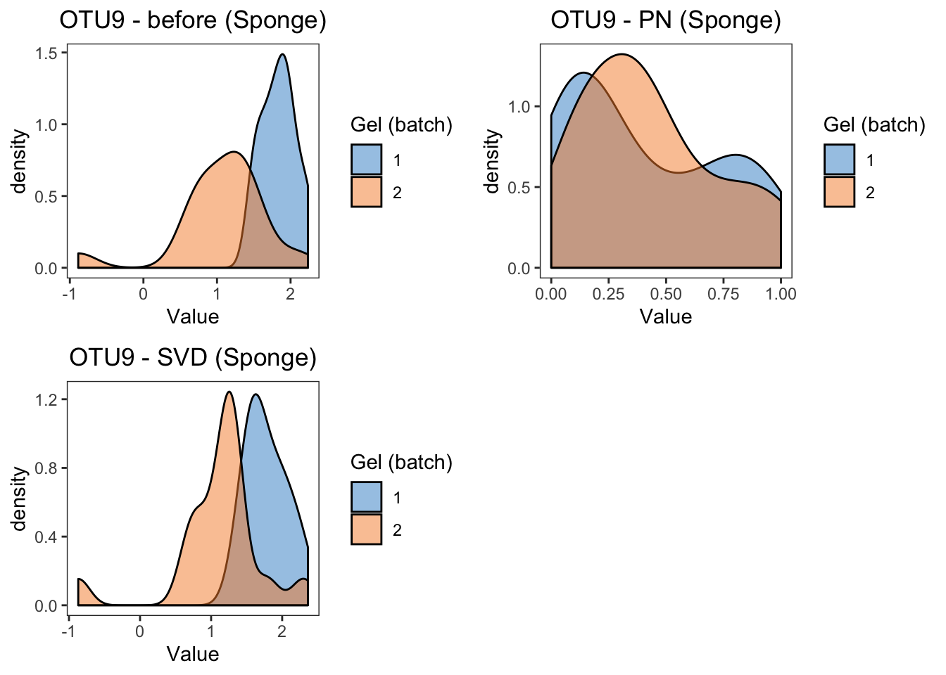
We can also assess the effect of batch in a linear model before and after batch correction.
# P-values
sponge.lm.before <- lm(sponge.tss.clr[ ,9] ~ sponge.trt + sponge.batch)
summary(sponge.lm.before)
##
## Call:
## lm(formula = sponge.tss.clr[, 9] ~ sponge.trt + sponge.batch)
##
## Residuals:
## Min 1Q Median 3Q Max
## -1.87967 -0.24705 0.04588 0.24492 1.00757
##
## Coefficients:
## Estimate Std. Error t value Pr(>|t|)
## (Intercept) 1.7849 0.1497 11.922 1.06e-12 ***
## sponge.trtE 0.1065 0.1729 0.616 0.543
## sponge.batch2 -0.7910 0.1729 -4.575 8.24e-05 ***
## ---
## Signif. codes: 0 '***' 0.001 '**' 0.01 '*' 0.05 '.' 0.1 ' ' 1
##
## Residual standard error: 0.489 on 29 degrees of freedom
## Multiple R-squared: 0.4236, Adjusted R-squared: 0.3839
## F-statistic: 10.66 on 2 and 29 DF, p-value: 0.0003391Before correction, the batch effect is statistically significant (P \(<\) 0.001), as indicated in the sponge.batch2 row.
sponge.lm.bmc <- lm(sponge.bmc[ ,9] ~ sponge.trt + sponge.batch)
summary(sponge.lm.bmc)
##
## Call:
## lm(formula = sponge.bmc[, 9] ~ sponge.trt + sponge.batch)
##
## Residuals:
## Min 1Q Median 3Q Max
## -1.87967 -0.24705 0.04588 0.24492 1.00757
##
## Coefficients:
## Estimate Std. Error t value Pr(>|t|)
## (Intercept) -5.323e-02 1.497e-01 -0.356 0.725
## sponge.trtE 1.065e-01 1.729e-01 0.616 0.543
## sponge.batch2 -3.925e-17 1.729e-01 0.000 1.000
##
## Residual standard error: 0.489 on 29 degrees of freedom
## Multiple R-squared: 0.01291, Adjusted R-squared: -0.05517
## F-statistic: 0.1896 on 2 and 29 DF, p-value: 0.8283After BMC correction, the batch effect is not statistically significant (P \(>\) 0.05), as indicated in the sponge.batch2 row.
The results from other batch correction methods are similar as BMC correction.
sponge.lm.combat <- lm(sponge.combat[ ,9] ~ sponge.trt + sponge.batch)
summary(sponge.lm.combat)

sponge.lm.limma <- lm(sponge.limma[ ,9] ~ sponge.trt + sponge.batch)
summary(sponge.lm.limma)

sponge.lm.percentile <- lm(sponge.percentile[ ,9] ~ sponge.trt + sponge.batch)
summary(sponge.lm.percentile)

sponge.lm.svd <- lm(sponge.svd[ ,9] ~ sponge.trt + sponge.batch)
summary(sponge.lm.svd)
In sponge data, the results of density plots and P-values of batch effects from linear models reach a consesus with boxplots, the difference between two batches are removed by BMC, ComBat, removeBatchEffect and percentile normalisation correction. We observe that percentile normalisation modifies the distribution of the samples from the two batches.
# ad data
# boxplot
ad.before.df <- data.frame(value = ad.clr[ ,1], batch = ad.batch)
ad.boxplot.before <- box_plot_fun(data = ad.before.df, x = ad.before.df$batch,
                                  y = ad.before.df$value,
                                  title = 'OTU12 - before (AD)',
                                  batch.legend.title = 'Date (batch)',
                                  x.angle = 45, x.hjust = 1)


ad.bmc.df <- data.frame(value = ad.bmc[ ,1], batch = ad.batch)
ad.boxplot.bmc <- box_plot_fun(data = ad.bmc.df,x = ad.bmc.df$batch,
                               y = ad.bmc.df$value,
                               title = 'OTU12 - BMC (AD)',
                               batch.legend.title = 'Date (batch)',
                               x.angle = 45, x.hjust = 1)


ad.combat.df <- data.frame(value = ad.combat[ ,1], batch = ad.batch)
ad.boxplot.combat <- box_plot_fun(data = ad.combat.df, x = ad.combat.df$batch,
                                  y = ad.combat.df$value,
                                  title = 'OTU12 - ComBat (AD)',
                                  batch.legend.title = 'Date (batch)',
                                  x.angle = 45, x.hjust = 1)

ad.limma.df <- data.frame(value = ad.limma[ ,1], batch = ad.batch)
ad.boxplot.limma <- box_plot_fun(data = ad.limma.df,x = ad.limma.df$batch,
                                 y = ad.limma.df$value,
                                 title = 'OTU12 - rBE (AD)',
                                 batch.legend.title = 'Date (batch)',
                                 x.angle = 45, x.hjust = 1)


ad.percentile.df <- data.frame(value = ad.percentile[ ,1], batch = ad.batch)
ad.boxplot.percentile <- box_plot_fun(data = ad.percentile.df,x = ad.percentile.df$batch,
                                      y = ad.percentile.df$value,
                                      title = 'OTU12 - PN (AD)',
                                      batch.legend.title = 'Date (batch)',
                                      x.angle = 45, x.hjust = 1)

ad.svd.df <- data.frame(value = ad.svd[ ,1], batch = ad.batch)
ad.boxplot.svd <- box_plot_fun(data = ad.svd.df,x = ad.svd.df$batch,
                               y = ad.svd.df$value,
                               title = 'OTU12 - SVD (AD)',
                               batch.legend.title = 'Date (batch)',
                               x.angle = 45, x.hjust = 1)

ad.ruv.df <- data.frame(value = ad.ruvIII[ ,1], batch = ad.batch)
ad.boxplot.ruv <- box_plot_fun(data = ad.ruv.df,x = ad.ruv.df$batch,
                               y = ad.ruv.df$value,
                               title = 'OTU12 - RUVIII (AD)',
                               batch.legend.title = 'Date (batch)',
x.angle = 45, x.hjust = 1)grid.arrange(ad.boxplot.before, ad.boxplot.bmc,
ad.boxplot.combat, ad.boxplot.limma, ncol = 2)
grid.arrange(ad.boxplot.before, ad.boxplot.percentile,
             ad.boxplot.svd, ad.boxplot.ruv, ncol = 2)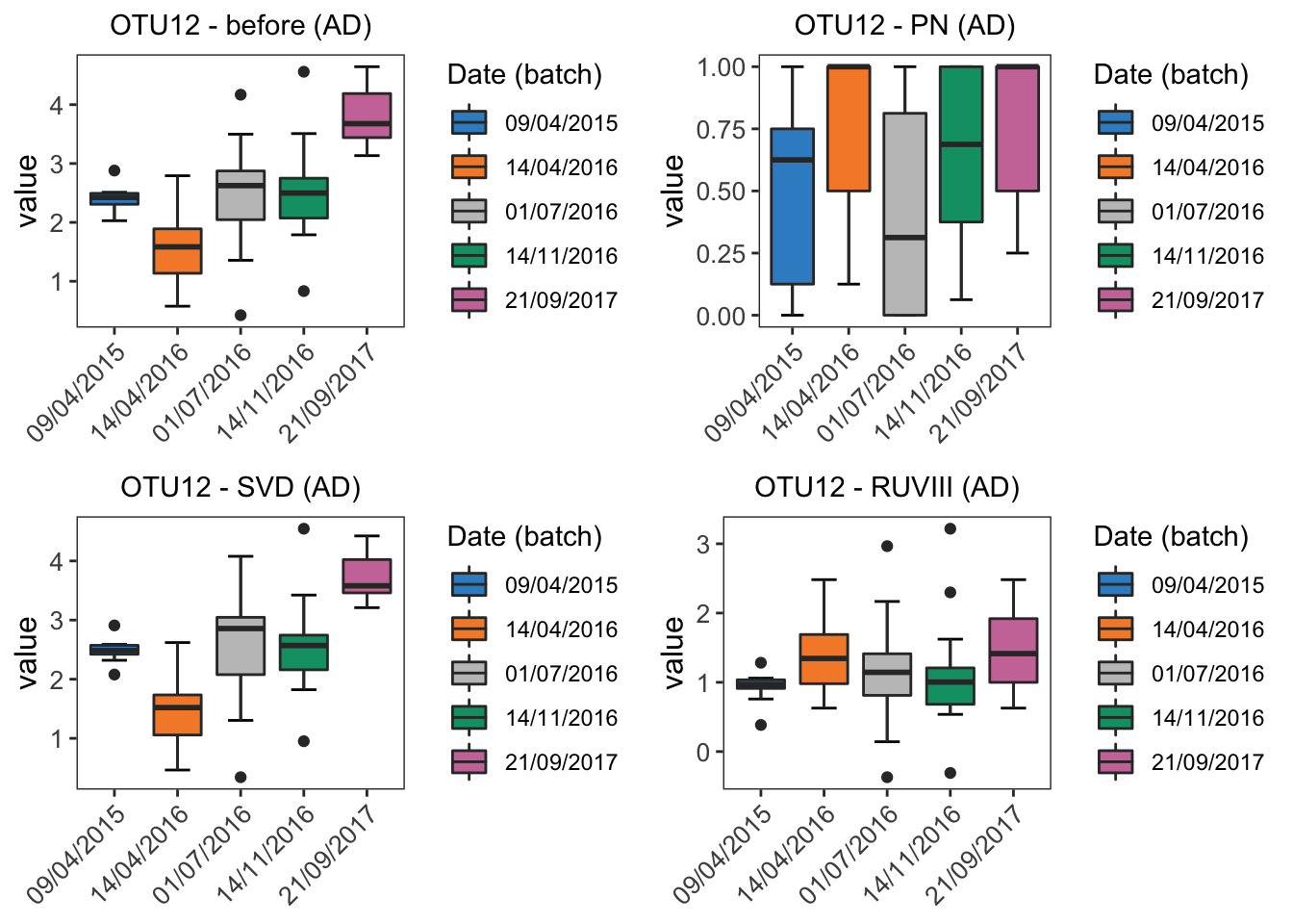
From the boxplots of OTU9 in AD data, the difference between five batches are removed by BMC, ComBat, removeBatchEffect and RUVIII correction. Among these methods, RUVIII did not remove as much batch difference as the other methods.
# density plot
# before
ad.dens.before <- ggplot(ad.before.df, aes(x = value, fill = batch)) +
  geom_density(alpha = 0.5) + scale_fill_manual(values = color.mixo(1:10)) +
  labs(title = 'OTU12 - before (AD)', x = 'Value', fill = 'Date (batch)') +
  theme_bw() + theme(plot.title = element_text(hjust = 0.5),
                     panel.grid = element_blank())

# BMC
ad.dens.bmc <- ggplot(ad.bmc.df, aes(x = value, fill = batch)) +
  geom_density(alpha = 0.5) + scale_fill_manual(values = color.mixo(1:10)) +
  labs(title = 'OTU12 - BMC (AD)', x = 'Value', fill = 'Date (batch)') +
  theme_bw() + theme(plot.title = element_text(hjust = 0.5),
                     panel.grid = element_blank())


# ComBat
ad.dens.combat <- ggplot(ad.combat.df, aes(x = value, fill = batch)) +
  geom_density(alpha = 0.5) + scale_fill_manual(values = color.mixo(1:10)) +
  labs(title = 'OTU12 - ComBat (AD)', x = 'Value', fill = 'Date (batch)') +
  theme_bw() + theme(plot.title = element_text(hjust = 0.5),
                     panel.grid = element_blank())


# removeBatchEffect
ad.dens.limma <- ggplot(ad.limma.df, aes(x = value, fill = batch)) +
  geom_density(alpha = 0.5) + scale_fill_manual(values = color.mixo(1:10)) +
  labs(title = 'OTU12 - rBE (AD)', x = 'Value', fill = 'Date (batch)') +
  theme_bw() + theme(plot.title = element_text(hjust = 0.5),
                     panel.grid = element_blank())


# percentile norm
ad.dens.percentile <- ggplot(ad.percentile.df, aes(x = value, fill = batch)) +
  geom_density(alpha = 0.5) + scale_fill_manual(values = color.mixo(1:10)) +
  labs(title = 'OTU12 - PN (AD)', x = 'Value', fill = 'Date (batch)') +
  theme_bw() + theme(plot.title = element_text(hjust = 0.5),
                     panel.grid = element_blank())


# SVD
ad.dens.svd <- ggplot(ad.svd.df, aes(x = value, fill = batch)) +
  geom_density(alpha = 0.5) + scale_fill_manual(values = color.mixo(1:10)) +
  labs(title = 'OTU12 - SVD (AD)', x = 'Value', fill = 'Date (batch)') +
  theme_bw() + theme(plot.title = element_text(hjust = 0.5),
                     panel.grid = element_blank())


# RUVIII
ad.dens.ruv <- ggplot(ad.ruv.df, aes(x = value, fill = batch)) +
  geom_density(alpha = 0.5) + scale_fill_manual(values = color.mixo(1:10)) +
  labs(title = 'OTU12 - RUVIII (AD)', x = 'Value', fill = 'Date (batch)') +
  theme_bw() + theme(plot.title = element_text(hjust = 0.5),
panel.grid = element_blank())grid.arrange(ad.dens.before, ad.dens.bmc,
ad.dens.combat, ad.dens.limma, ncol = 2)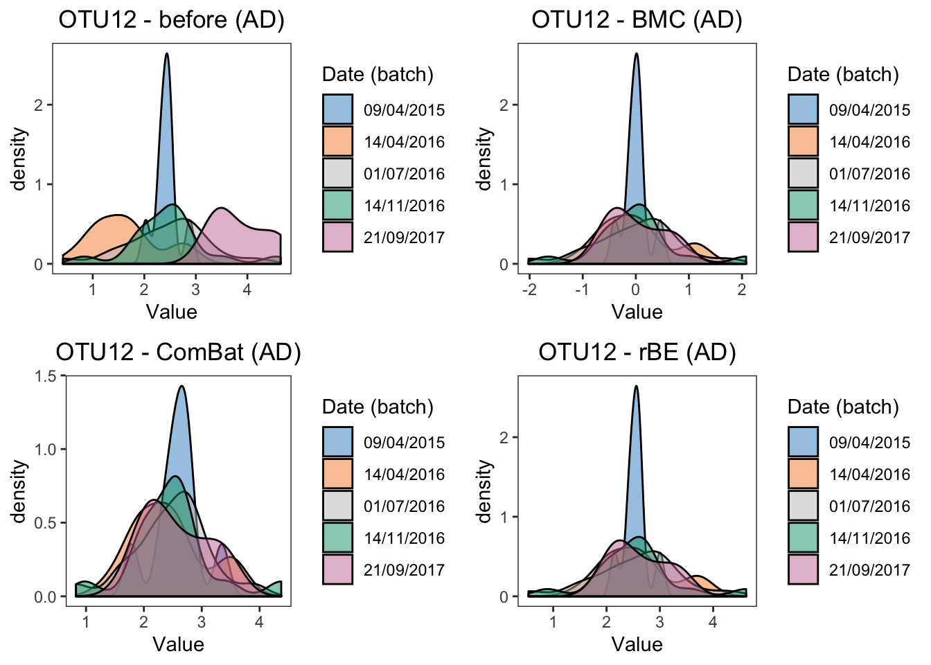
grid.arrange(ad.dens.before, ad.dens.percentile,
             ad.dens.svd, ad.dens.ruv, ncol = 2)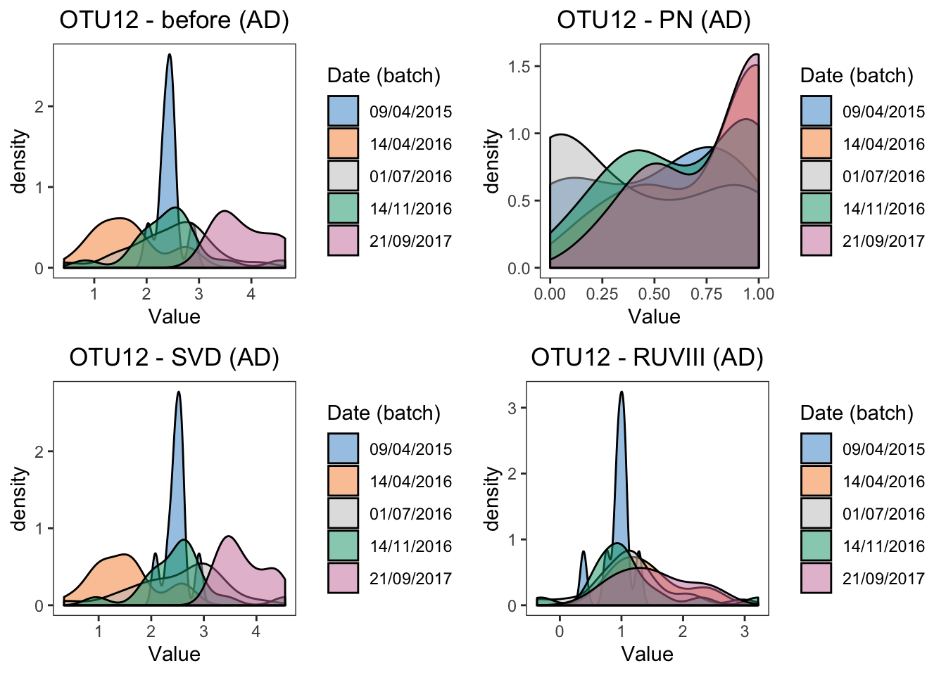
Similar as sponge data, we can also assess the batch effect in AD data using linear model.
#p-values
ad.lm.before <- lm(ad.clr[ ,1] ~ ad.trt + ad.batch)
anova(ad.lm.before)
## Analysis of Variance Table
##
## Response: ad.clr[, 1]
## Df Sum Sq Mean Sq F value Pr(>F)
## ad.trt 1 1.460 1.4605 3.1001 0.08272 .
## ad.batch 4 32.889 8.2222 17.4532 6.168e-10 ***
## Residuals 69 32.506 0.4711
## ---
## Signif. codes: 0 '***' 0.001 '**' 0.01 '*' 0.05 '.' 0.1 ' ' 1#summary(ad.lm.before)Before correction, the batch effect is statistically significant (P \(<\) 0.001), as indicated in the ad.batch row.
ad.lm.bmc <- lm(ad.bmc[ ,1] ~ ad.trt + ad.batch)
anova(ad.lm.bmc)
## Analysis of Variance Table
##
## Response: ad.bmc[, 1]
## Df Sum Sq Mean Sq F value Pr(>F)
## ad.trt 1 0.631 0.63084 1.3391 0.2512
## ad.batch 4 0.036 0.00893 0.0190 0.9993
## Residuals 69 32.506 0.47110#summary(ad.lm.bmc)After BMC correction, the batch effect is not statistically significant (P \(>\) 0.05), as indicated in the ad.batch row.The results from other batch correction methods are similar as BMC correction.
ad.lm.combat <- lm(ad.combat[ ,1] ~ ad.trt + ad.batch)
anova(ad.lm.combat)
#summary(ad.lm.combat)

ad.lm.limma <- lm(ad.limma[ ,1] ~ ad.trt + ad.batch)
anova(ad.lm.limma)
#summary(ad.lm.limma)

ad.lm.percentile <- lm(ad.percentile[ ,1] ~ ad.trt + ad.batch)
anova(ad.lm.percentile)
#summary(ad.lm.percentile)

ad.lm.svd <- lm(ad.svd[ ,1] ~ ad.trt + ad.batch)
anova(ad.lm.svd)
#summary(ad.lm.svd)


ad.lm.ruv <- lm(ad.ruvIII[ ,1] ~ ad.trt + ad.batch)
anova(ad.lm.ruv)
#summary(ad.lm.ruv)
The results of density plots and P-values of batch effects from linear models reach a consesus with boxplots, the difference between two batches are removed by BMC, ComBat, removeBatchEffect and RUVIII correction.
4.1.3 RLE plots
In sponge data, we group the samples according to the tissue (choanosome / ectosome) and generate two RLE plots respectively in all datasets before and after batch correction with different methods:
# sponge data
# BMC
sponge.bmc_c <- sponge.bmc[sponge.trt == 'C', ]
sponge.bmc_e <- sponge.bmc[sponge.trt == 'E', ]

# ComBat
sponge.combat_c <- sponge.combat[sponge.trt == 'C', ]
sponge.combat_e <- sponge.combat[sponge.trt == 'E', ]

# rBE
sponge.limma_c <- sponge.limma[sponge.trt == 'C', ]
sponge.limma_e <- sponge.limma[sponge.trt == 'E', ]

# PN
sponge.percentile_c <- sponge.percentile[sponge.trt == 'C', ]
sponge.percentile_e <- sponge.percentile[sponge.trt == 'E', ]

# SVD
sponge.svd_c <- sponge.svd[sponge.trt == 'C', ]
sponge.svd_e <- sponge.svd[sponge.trt == 'E', ] par(mfrow = c(2,3), mai = c(0.4,0.6,0.3,0.1))
RleMicroRna2(object = t(sponge.before_c), batch = sponge.batch_c,
maintitle = 'Sponge: before (choanosome)', title.cex = 1)
RleMicroRna2(object = t(sponge.bmc_c), batch = sponge.batch_c,
maintitle = 'Sponge: BMC (choanosome)', title.cex = 1)
RleMicroRna2(object = t(sponge.combat_c), batch = sponge.batch_c,
maintitle = 'Sponge: ComBat (choanosome)', title.cex = 1)
RleMicroRna2(object = t(sponge.limma_c), batch = sponge.batch_c,
maintitle = 'Sponge: rBE (choanosome)', title.cex = 1)
RleMicroRna2(object = t(sponge.percentile_c), batch = sponge.batch_c,
maintitle = 'Sponge: PN (choanosome)', title.cex = 1)
RleMicroRna2(object = t(sponge.svd_c), batch = sponge.batch_c,
maintitle = 'Sponge: SVD (choanosome)', title.cex = 1)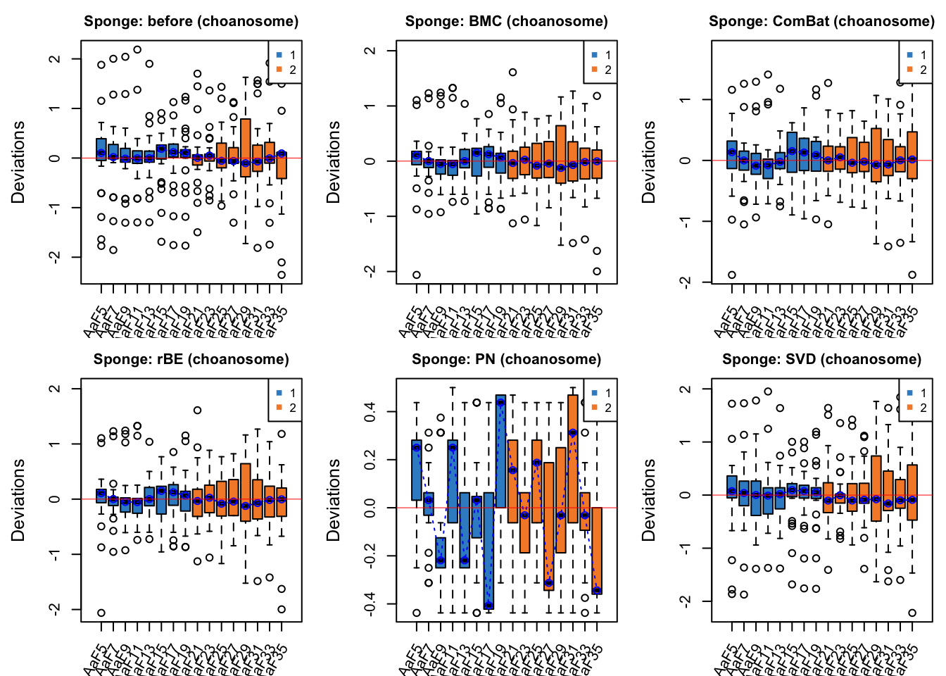
par(mfrow = c(1,1))In tissue choanosome of sponge data, the batch effect before correction is not obvious as all medians of samples are close to zero, but Gel2 has a greater interquartile range (IQR) than the other samples. Percentile normalisation increased batch effects, as the samples after correction are deviated from zero and the IQR is increased. Among other methods, the IQR of all the box plots (samples) from different batches is consistent after ComBat correction.
par(mfrow = c(2,3), mai = c(0.4,0.6,0.3,0.1))

RleMicroRna2(object = t(sponge.before_e), batch = sponge.batch_e,
             maintitle = 'Sponge: before (ectosome)', title.cex = 1)

RleMicroRna2(object = t(sponge.bmc_e), batch = sponge.batch_e,
             maintitle = 'Sponge: BMC (ectosome)', title.cex = 1)

RleMicroRna2(object = t(sponge.combat_e), batch = sponge.batch_e,
             maintitle = 'Sponge: ComBat (ectosome)', title.cex = 1)

RleMicroRna2(object = t(sponge.limma_e), batch = sponge.batch_e,
             maintitle = 'Sponge: rBE (ectosome)', title.cex = 1)

RleMicroRna2(object = t(sponge.percentile_e), batch = sponge.batch_e,
             maintitle = 'Sponge: PN (ectosome)', title.cex = 1)

RleMicroRna2(object = t(sponge.svd_e), batch = sponge.batch_e,
             maintitle = 'Sponge: SVD (ectosome)', title.cex = 1)
par(mfrow = c(1,1))In tissue ectosome of sponge data, batch effect is not easily detected, but percentile normalisation increased batch variation.
In AD data, we group the samples according to the inital phenol concentration (0-0.5 g/L / 1-2 g/L) and generate two RLE plots respectively in all datasets before and after batch correction, as sponge data:
# ad data
# BMC
ad.bmc_05 <- ad.bmc[ad.trt == '0-0.5', ]
ad.bmc_2 <- ad.bmc[ad.trt == '1-2', ]

# ComBat
ad.combat_05 <- ad.combat[ad.trt == '0-0.5', ]
ad.combat_2 <- ad.combat[ad.trt == '1-2', ]

# rBE
ad.limma_05 <- ad.limma[ad.trt == '0-0.5', ]
ad.limma_2 <- ad.limma[ad.trt == '1-2', ]

# PN
ad.percentile_05 <- ad.percentile[ad.trt == '0-0.5', ]
ad.percentile_2 <- ad.percentile[ad.trt == '1-2', ]

# SVD
ad.svd_05 <- ad.svd[ad.trt == '0-0.5', ]
ad.svd_2 <- ad.svd[ad.trt == '1-2', ]

# RUVIII
ad.ruv_05 <- ad.ruvIII[ad.trt == '0-0.5', ]
ad.ruv_2 <- ad.ruvIII[ad.trt == '1-2', ]par(mfrow = c(2,2), mai = c(0.5,0.8,0.3,0.1))
RleMicroRna2(object = t(ad.before_05), batch = ad.batch_05,
maintitle = 'AD: before (0-0.5 g/L)', legend.cex = 0.4,
cex.xaxis = 0.5)
RleMicroRna2(object = t(ad.bmc_05), batch = ad.batch_05,
maintitle = 'AD: BMC (0-0.5 g/L)', legend.cex = 0.4,
cex.xaxis = 0.5)
RleMicroRna2(object = t(ad.combat_05), batch = ad.batch_05,
maintitle = 'AD: ComBat (0-0.5 g/L)', legend.cex = 0.4,
cex.xaxis = 0.5)
RleMicroRna2(object = t(ad.limma_05), batch = ad.batch_05,
maintitle = 'AD: rBE (0-0.5 g/L)', legend.cex = 0.4,
cex.xaxis = 0.5)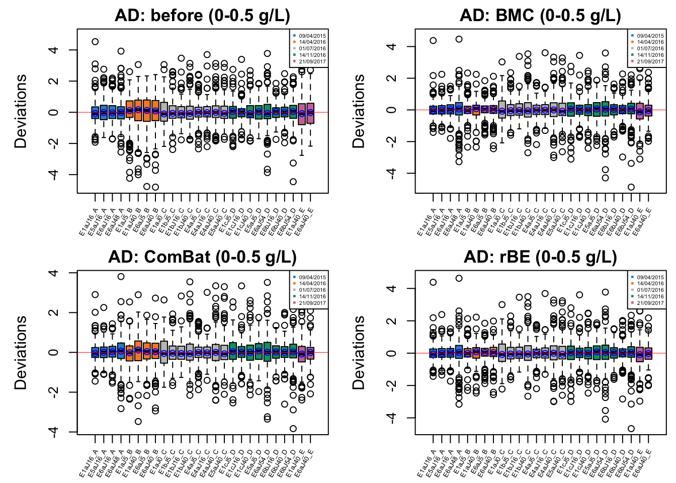
RleMicroRna2(object = t(ad.percentile_05), batch = ad.batch_05,
             maintitle = 'AD: PN (0-0.5 g/L)', legend.cex = 0.4,
             cex.xaxis = 0.5)

RleMicroRna2(object = t(ad.svd_05), batch = ad.batch_05,
             maintitle = 'AD: SVD (0-0.5 g/L)', legend.cex = 0.4,
             cex.xaxis = 0.5)

RleMicroRna2(object = t(ad.ruv_05), batch = ad.batch_05,
             maintitle = 'AD: RUVIII (0-0.5 g/L)', legend.cex = 0.4,
             cex.xaxis = 0.5)

par(mfrow = c(1,1))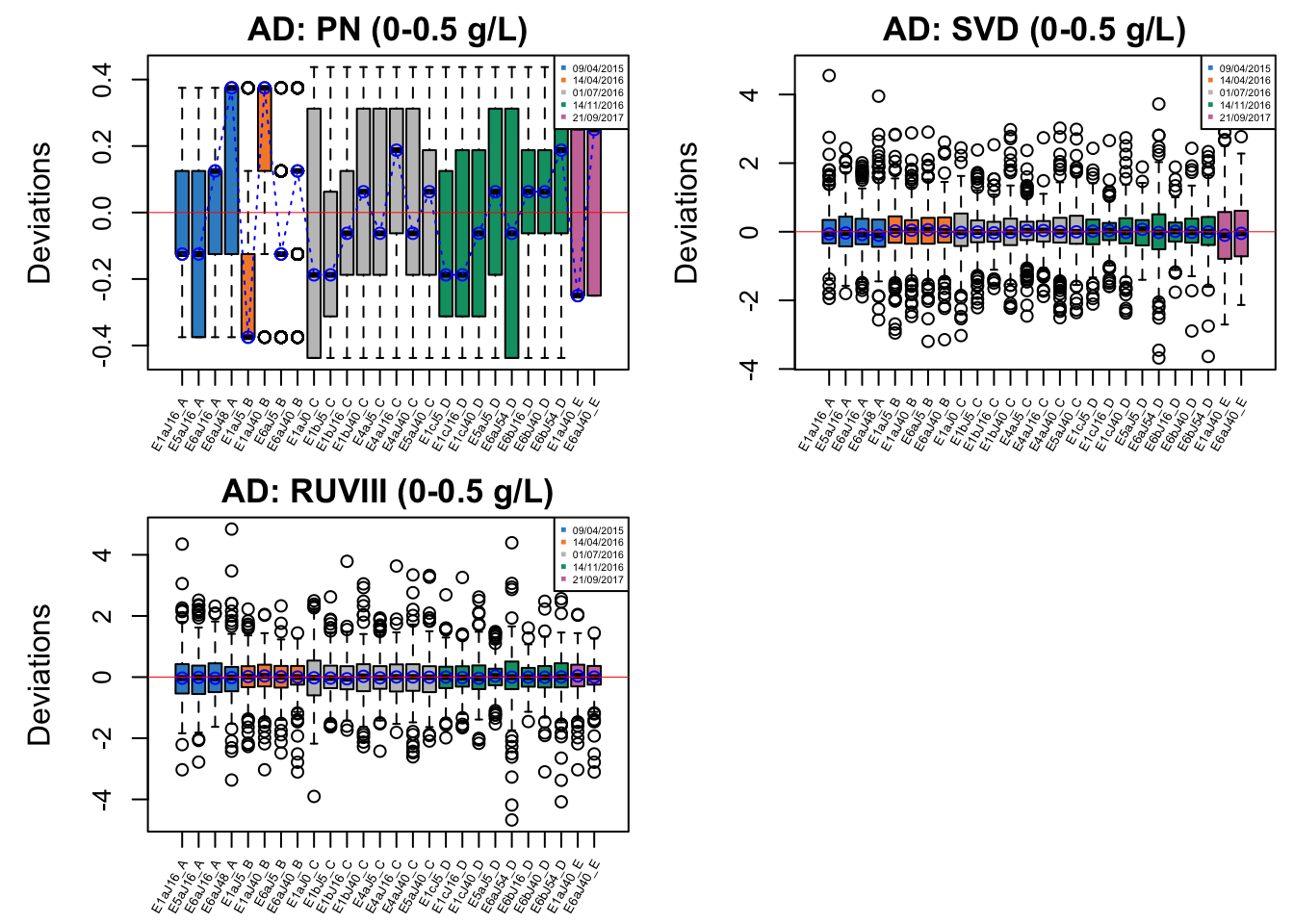
In AD data with initial phenol concentration between 0-0.5 g/L, batch effect is not easily detected, but percentile normalisation increased batch variation.
par(mfrow = c(2,2), mai = c(0.35,0.8,0.3,0.1))

RleMicroRna2(object = t(ad.before_2), batch = ad.batch_2,
             maintitle = 'AD: before (1-2 g/L)', legend.cex = 0.4,
             cex.xaxis = 0.3)

RleMicroRna2(object = t(ad.bmc_2), batch = ad.batch_2,
             maintitle = 'AD: BMC (1-2 g/L)', legend.cex = 0.4,
             cex.xaxis = 0.3)

RleMicroRna2(object = t(ad.combat_2), batch = ad.batch_2,
             maintitle = 'AD: ComBat (1-2 g/L)', legend.cex = 0.4,
             cex.xaxis = 0.3)

RleMicroRna2(object = t(ad.limma_2), batch = ad.batch_2,
             maintitle = 'AD: rBE (1-2 g/L)', legend.cex = 0.4,
             cex.xaxis = 0.3)
RleMicroRna2(object = t(ad.percentile_2), batch = ad.batch_2,
             maintitle = 'AD: PN (1-2 g/L)', legend.cex = 0.4,
             cex.xaxis = 0.3)

RleMicroRna2(object = t(ad.svd_2), batch = ad.batch_2,
             maintitle = 'AD: SVD (1-2 g/L)', legend.cex = 0.4,
             cex.xaxis = 0.3)

RleMicroRna2(object = t(ad.ruv_2), batch = ad.batch_2,
             maintitle = 'AD: RUVIII (1-2 g/L)', legend.cex = 0.4,
             cex.xaxis = 0.3)

par(mfrow = c(1,1))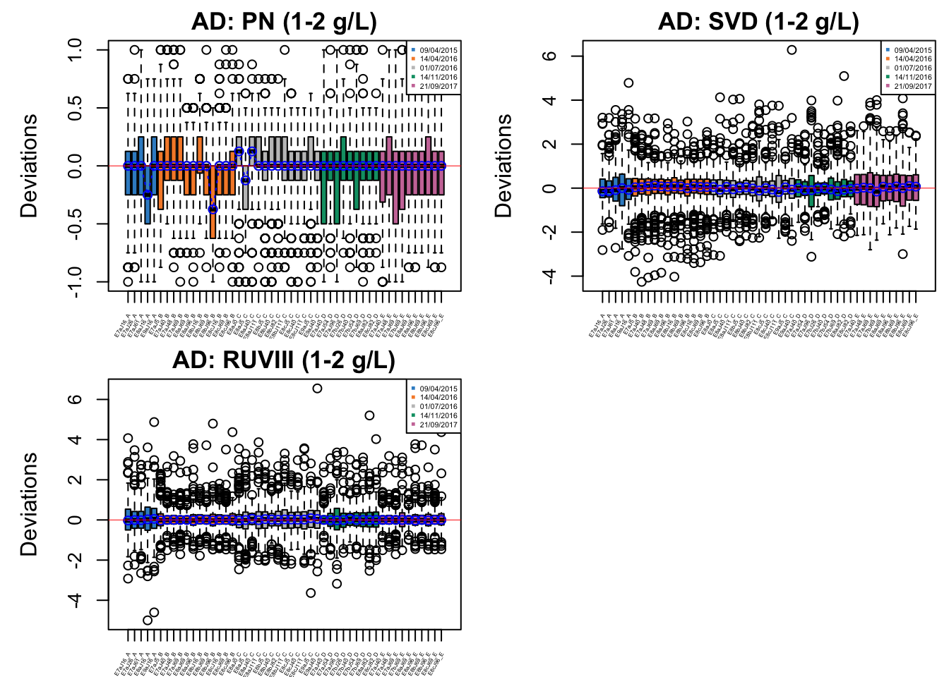
In AD data with initial phenol concentration between 1-2 g/L, batch effect is not easily detected, but percentile normalisation increased batch variation.
4.1.4 Heatmap
We use the heatmap to visualise data clusters. Samples clustered by batches instead of treatments indicate a batch effect.
# Sponge data
# before
sponge.tss.clr.scale <- scale(sponge.tss.clr, center = T, scale = T)
# scale on OTUs
sponge.tss.clr.scale <- scale(t(sponge.tss.clr.scale), center = T, scale = T)
# scale on samples

sponge.anno_col <- data.frame(Batch = sponge.batch, Tissue = sponge.trt)
sponge.anno_metabo_colors <- list(Batch = c('1' = '#388ECC', '2' = '#F68B33'),
                                 Tissue = c(C = '#F0E442', E = '#D55E00'))


pheatmap(sponge.tss.clr.scale,
         scale = 'none',
         cluster_rows = F,
         cluster_cols = T,
         fontsize_row = 5, fontsize_col = 8,
         fontsize = 8,
         clustering_distance_rows = 'euclidean',
         clustering_method = 'ward.D',
         treeheight_row = 30,
         annotation_col = sponge.anno_col,
         annotation_colors = sponge.anno_metabo_colors,
         border_color = 'NA',
         main = 'Sponge data - before')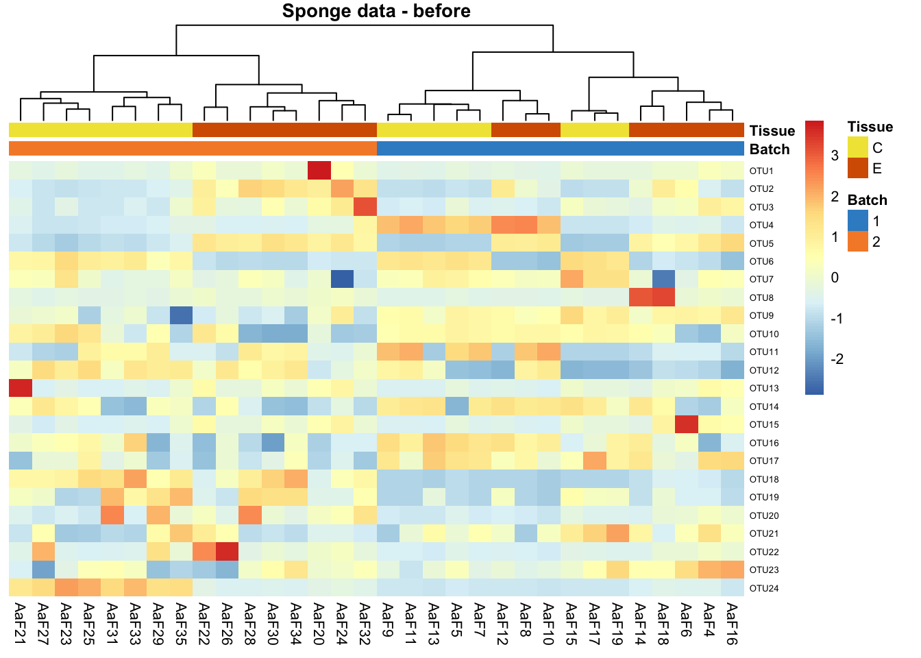
Before correction, samples in sponge data are preferentially clustered by batch instead of tissue type, indicating a batch effect.
# ComBat
sponge.combat.scale <- scale(sponge.combat, center = T, scale = T)
# scale on OTUs
sponge.combat.scale <- scale(t(sponge.combat.scale), center = T, scale = T)
# scale on samples

pheatmap(sponge.combat.scale,
         scale = 'none',
         cluster_rows = F,
         cluster_cols = T,
         fontsize_row = 5, fontsize_col = 8,
         fontsize = 8,
         clustering_distance_rows = 'euclidean',
         clustering_method = 'ward.D',
         treeheight_row = 30,
         annotation_col = sponge.anno_col,
         annotation_colors = sponge.anno_metabo_colors,
         border_color = 'NA',
         main = 'Sponge data - ComBat')
After batch correction with ComBat, the data are clustered by tissues rather than batches, therefore, ComBat not only removed batch effects, but also disengaged the effect of interest. The results from batch correction with other methods are similar.
# BMC
sponge.bmc.scale <- scale(sponge.bmc, center = T, scale = T)
# scale on OTUs
sponge.bmc.scale <- scale(t(sponge.bmc.scale), center = T, scale = T)
# scale on samples

pheatmap(sponge.bmc.scale,
         scale = 'none',
         cluster_rows = F,
         cluster_cols = T,
         fontsize_row = 5, fontsize_col = 8,
         fontsize = 8,
         clustering_distance_rows = 'euclidean',
         clustering_method = 'ward.D',
         treeheight_row = 30,
         annotation_col = sponge.anno_col,
         annotation_colors = sponge.anno_metabo_colors,
         border_color = 'NA',
         main = 'Sponge data - BMC')


# removeBatchEffect
sponge.limma.scale <- scale(sponge.limma, center = T, scale = T)
# scale on OTUs
sponge.limma.scale <- scale(t(sponge.limma.scale), center = T, scale = T)
# scale on samples

pheatmap(sponge.limma.scale,
         scale = 'none',
         cluster_rows = F,
         cluster_cols = T,
         fontsize_row = 5, fontsize_col = 8,
         fontsize = 8,
         clustering_distance_rows = 'euclidean',
         clustering_method = 'ward.D',
         treeheight_row = 30,
         annotation_col = sponge.anno_col,
         annotation_colors = sponge.anno_metabo_colors,
         border_color = 'NA',
         main = 'Sponge data - removeBatchEffect')

# percentile normalisation
sponge.percentile.scale <- scale(sponge.percentile, center = T, scale = T)
# scale on OTUs
sponge.percentile.scale <- scale(t(sponge.percentile.scale), center = T, scale = T)
# scale on samples

pheatmap(sponge.percentile.scale,
         scale = 'none',
         cluster_rows = F,
         cluster_cols = T,
         fontsize_row = 5, fontsize_col = 8,
         fontsize = 8,
         clustering_distance_rows = 'euclidean',
         clustering_method = 'ward.D',
         treeheight_row = 30,
         annotation_col = sponge.anno_col,
         annotation_colors = sponge.anno_metabo_colors,
         border_color = 'NA',
         main = 'Sponge data - percentile norm')


# SVD
sponge.svd.scale <- scale(sponge.svd, center = T, scale = T)
# scale on OTUs
sponge.svd.scale <- scale(t(sponge.svd.scale), center = T, scale = T)
# scale on samples

pheatmap(sponge.svd.scale,
         scale = 'none',
         cluster_rows = F,
         cluster_cols = T,
         fontsize_row = 5, fontsize_col = 8,
         fontsize = 8,
         clustering_distance_rows = 'euclidean',
         clustering_method = 'ward.D',
         treeheight_row = 30,
         annotation_col = sponge.anno_col,
         annotation_colors = sponge.anno_metabo_colors,
         border_color = 'NA',
         main = 'Sponge data - SVD')
In the heatmap of AD data before batch correction, samples within batch 14/04/2016 are clustered and distinct from other samples, indicating a batch effect.
# AD data
# before
ad.clr.scale <- scale(ad.clr, center = T, scale = T) # scale on OTUs
ad.clr.scale <- scale(t(ad.clr.scale), center = T, scale = T) # scale on samples

ad.anno_col <- data.frame(Batch = ad.batch, Treatment = ad.trt)
ad.anno_metabo_colors <- list(Batch = c('09/04/2015' = '#388ECC',
                                       '14/04/2016' = '#F68B33',
                                       '01/07/2016' = '#C2C2C2',
                                       '14/11/2016' = '#009E73',
                                       '21/09/2017' = '#CC79A7'),
                             Treatment = c('0-0.5' = '#0072B2', '1-2' = '#999999'))


pheatmap(ad.clr.scale,
         scale = 'none',
         cluster_rows = F,
         cluster_cols = T,
         fontsize_row = 4, fontsize_col = 6,
         fontsize = 8,
         clustering_distance_rows = 'euclidean',
         clustering_method = 'ward.D',
         treeheight_row = 30,
         annotation_col = ad.anno_col,
         annotation_colors = ad.anno_metabo_colors,
         border_color = 'NA',
         main = 'AD data - before')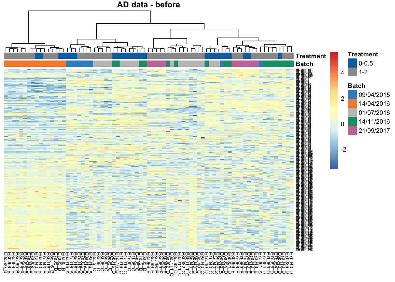
# removeBatchEffect
ad.limma.scale <- scale(ad.limma, center = T, scale = T) # scale on OTUs
ad.limma.scale <- scale(t(ad.limma.scale), center = T, scale = T) # scale on samples

pheatmap(ad.limma.scale,
         scale = 'none',
         cluster_rows = F,
         cluster_cols = T,
         fontsize_row = 4, fontsize_col = 6,
         fontsize = 8,
         clustering_distance_rows = 'euclidean',
         clustering_method = 'ward.D',
         treeheight_row = 30,
         annotation_col = ad.anno_col,
         annotation_colors = ad.anno_metabo_colors,
         border_color = 'NA',
         main = 'AD data - removeBatchEffect')
After batch correction with removeBatchEffect, the data are almost clustered by treatments rather than batches, therefore, removeBatchEffect not only removed batch effects, but also disengaged the treatment effects. The results from batch correction with other methods are similar.
# BMC
ad.bmc.scale <- scale(ad.bmc, center = T, scale = T) # scale on OTUs
ad.bmc.scale <- scale(t(ad.bmc.scale), center = T, scale = T) # scale on samples

pheatmap(ad.bmc.scale,
         scale = 'none',
         cluster_rows = F,
         cluster_cols = T,
         fontsize_row = 4, fontsize_col = 6,
         fontsize = 8,
         clustering_distance_rows = 'euclidean',
         clustering_method = 'ward.D',
         treeheight_row = 30,
         annotation_col = ad.anno_col,
         annotation_colors = ad.anno_metabo_colors,
         border_color = 'NA',
         main = 'AD data - BMC')

# ComBat
ad.combat.scale <- scale(ad.combat, center = T, scale = T) # scale on OTUs
ad.combat.scale <- scale(t(ad.combat.scale), center = T, scale = T) # scale on samples

pheatmap(ad.combat.scale,
         scale = 'none',
         cluster_rows = F,
         cluster_cols = T,
         fontsize_row = 4, fontsize_col = 6,
         fontsize = 8,
         clustering_distance_rows = 'euclidean',
         clustering_method = 'ward.D',
         treeheight_row = 30,
         annotation_col = ad.anno_col,
         annotation_colors = ad.anno_metabo_colors,
         border_color = 'NA',
         main = 'AD data - ComBat')


# percentile normalisation
ad.percentile.scale <- scale(ad.percentile, center = T, scale = T) # scale on OTUs
ad.percentile.scale <- scale(t(ad.percentile.scale), center = T, scale = T) # scale on samples

pheatmap(ad.percentile.scale,
         scale = 'none',
         cluster_rows = F,
         cluster_cols = T,
         fontsize_row = 4, fontsize_col = 6,
         fontsize = 8,
         clustering_distance_rows = 'euclidean',
         clustering_method = 'ward.D',
         treeheight_row = 30,
         annotation_col = ad.anno_col,
         annotation_colors = ad.anno_metabo_colors,
         border_color = 'NA',
         main = 'AD data - percentile norm')

# SVD
ad.svd.scale <- scale(ad.svd, center = T, scale = T) # scale on OTUs
ad.svd.scale <- scale(t(ad.svd.scale), center = T, scale = T) # scale on samples

pheatmap(ad.svd.scale,
         scale = 'none',
         cluster_rows = F,
         cluster_cols = T,
         fontsize_row = 4, fontsize_col = 6,
         fontsize = 8,
         clustering_distance_rows = 'euclidean',
         clustering_method = 'ward.D',
         treeheight_row = 30,
         annotation_col = ad.anno_col,
         annotation_colors = ad.anno_metabo_colors,
         border_color = 'NA',
         main = 'AD data - SVD')


# RUVIII
ad.ruv.scale <- scale(ad.ruvIII, center = T, scale = T) # scale on OTUs
ad.ruv.scale <- scale(t(ad.ruv.scale), center = T, scale = T) # scale on samples

pheatmap(ad.ruv.scale,
         scale = 'none',
         cluster_rows = F,
         cluster_cols = T,
         fontsize_row = 4, fontsize_col = 6,
         fontsize = 8,
         clustering_distance_rows = 'euclidean',
         clustering_method = 'ward.D',
         treeheight_row = 30,
         annotation_col = ad.anno_col,
         annotation_colors = ad.anno_metabo_colors,
         border_color = 'NA',
         main = 'AD data - RUVIII')
4.2 Variance calculation
Compared to diagnostic plots, quantitative approaches are more objective and direct. The evaluation is done quantitatively before and after batch effect removal and the biological (treatment) effect must also be assessed before and after the batch effect correction to ensure it has been preserved.
4.2.1 Linear model per variable
The variance explained by batch or treatment per OTU can be calculated by a linear model. Box plots can then be used to visualise the variance calculated from each OTU. Following batch effect correction, the percentage of variance explained by the treatment should be greater than the batch.
We use a function fitExtractVarPartModel to calculate and extract the variance of batch and treatment per OTU.
# Sponge data
sponge.form <- ~ sponge.trt + sponge.batch
sponge.info <- as.data.frame(cbind(rownames(sponge.tss.clr), sponge.trt, sponge.batch))
rownames(sponge.info) <- rownames(sponge.tss.clr)

# before
sponge.varPart.before <- fitExtractVarPartModel(exprObj = t(sponge.tss.clr),
                                                formula = sponge.form,
                                                data = sponge.info)

# BMC
sponge.varPart.bmc <- fitExtractVarPartModel(exprObj = t(sponge.bmc),
                                             formula = sponge.form,
                                             data = sponge.info)

# combat
sponge.varPart.combat <- fitExtractVarPartModel(exprObj = t(sponge.combat),
                                                formula = sponge.form,
                                                data = sponge.info)

# removeBatchEffect
sponge.varPart.limma <- fitExtractVarPartModel(exprObj = t(sponge.limma),
                                               formula = sponge.form,
                                               data = sponge.info)

# percentile normalisation
sponge.varPart.percentile <- fitExtractVarPartModel(exprObj = t(sponge.percentile),
                                                    formula = sponge.form,
                                                    data = sponge.info)

# svd
sponge.varPart.svd <- fitExtractVarPartModel(exprObj = t(sponge.svd),
                                             formula = sponge.form,
                                             data = sponge.info)
# extract the variance of trt and batch
# before
sponge.varmat.before <- as.matrix(sponge.varPart.before[ ,1:2])
# BMC
sponge.varmat.bmc <- as.matrix(sponge.varPart.bmc[ ,1:2])
# ComBat
sponge.varmat.combat <- as.matrix(sponge.varPart.combat[ ,1:2])
# removeBatchEffect
sponge.varmat.limma <- as.matrix(sponge.varPart.limma[ ,1:2])
# percentile normalisation
sponge.varmat.percentile <- as.matrix(sponge.varPart.percentile[ ,1:2])
# SVD
sponge.varmat.svd <- as.matrix(sponge.varPart.svd[ ,1:2])
# merge results
sponge.variance <- c(as.vector(sponge.varmat.before), as.vector(sponge.varmat.bmc),
as.vector(sponge.varmat.combat), as.vector(sponge.varmat.limma),
as.vector(sponge.varmat.percentile), as.vector(sponge.varmat.svd))
# add batch, trt and methods info
sponge.variance <- cbind(variance = sponge.variance,
Type = rep(c('Tissue', 'Batch'), each = ncol(sponge.tss.clr)),
method = rep(c('Before', 'BMC', 'ComBat', 'rBE',
'PN', 'SVD'), each = 2*ncol(sponge.tss.clr)))
# reorder levels
sponge.variance <- as.data.frame(sponge.variance)
sponge.variance$method <- factor(sponge.variance$method,
levels = unique(sponge.variance$method))
sponge.variance$variance <- as.numeric(as.character(sponge.variance$variance))
ggplot(sponge.variance, aes(x = Type, y = variance, fill = Type)) +
geom_boxplot() + facet_grid(cols = vars(method)) + theme_bw() +
theme(axis.text.x = element_text(angle = 60, hjust = 1),
strip.text = element_text(size = 12), panel.grid = element_blank(),
axis.text = element_text(size = 12), axis.title = element_text(size = 15),
legend.title = element_text(size = 15), legend.text = element_text(size = 12)) +
labs(x = 'Type', y = 'Proportion Variance', name = 'Type') + ylim(0,1)
BMC, ComBat and removeBatchEffect successfully removed batch variation while preserving treatment variation, but SVD performed poorly. Percentile normalisation preserved sufficient treatment variation, but removed less batch effect variation than BMC, ComBat and removeBatchEffect. Percentile normalisation used percentiles instead of actual values. This leads to information loss. Moreover, it was designed for case-control microbiome studies, which differ from our example studies. This method would therefore be more effective with control samples in each batch. SVD was inefficient at targeting batch effects, as it assumes that batch effects cause the largest variation in the data and should therefore appear as the first component. However, in sponge data the batch effect is mainly present on the second component as was shown in PCA sample plots with density, which results in a miscorrection of batch effects.
We also calculate the variance for AD data.
# AD data
ad.form <- ~ ad.trt + ad.batch
ad.info <- as.data.frame(cbind(rownames(ad.clr), ad.trt,ad.batch))
rownames(ad.info) <- rownames(ad.clr)

# before
ad.varPart.before <- fitExtractVarPartModel(exprObj = t(ad.clr),
                                            formula = ad.form, data = ad.info)

# BMC
ad.varPart.bmc <- fitExtractVarPartModel(exprObj = t(ad.bmc),
                                         formula = ad.form, data = ad.info)

# combat
ad.varPart.combat <- fitExtractVarPartModel(exprObj = t(ad.combat),
                                            formula = ad.form, data = ad.info)

# removeBatchEffect
ad.varPart.limma <- fitExtractVarPartModel(exprObj = t(ad.limma),
                                           formula = ad.form, data = ad.info)

# percentile normalisation
ad.varPart.percentile <- fitExtractVarPartModel(exprObj = t(ad.percentile),
                                                formula = ad.form, data = ad.info)

# svd
ad.varPart.svd <- fitExtractVarPartModel(exprObj = t(ad.svd),
                                         formula = ad.form, data = ad.info)

# ruv
ad.varPart.ruv <- fitExtractVarPartModel(exprObj = t(ad.ruvIII),
                                         formula = ad.form, data = ad.info)
# extract the variance of trt and batch
# before
ad.varmat.before <- as.matrix(ad.varPart.before[ ,1:2])
# BMC
ad.varmat.bmc <- as.matrix(ad.varPart.bmc[ ,1:2])
# ComBat
ad.varmat.combat <- as.matrix(ad.varPart.combat[ ,1:2])
# removeBatchEffect
ad.varmat.limma <- as.matrix(ad.varPart.limma[ ,1:2])
# percentile normalisation
ad.varmat.percentile <- as.matrix(ad.varPart.percentile[ ,1:2])
# SVD
ad.varmat.svd <- as.matrix(ad.varPart.svd[ ,1:2])
# RUVIII
ad.varmat.ruv <- as.matrix(ad.varPart.ruv[ ,1:2])
# merge results
ad.variance <- c(as.vector(ad.varmat.before), as.vector(ad.varmat.bmc),
as.vector(ad.varmat.combat), as.vector(ad.varmat.limma),
as.vector(ad.varmat.percentile), as.vector(ad.varmat.svd),
as.vector(ad.varmat.ruv))
# add batch, trt and methods info
ad.variance <- cbind(variance = ad.variance,
Type = rep(c( 'Treatment', 'Batch'), each = ncol(ad.clr)),
method = rep(c('Before', 'BMC', 'ComBat', 'rBE', 'PN',
'SVD', 'RUVIII'), each = 2*ncol(ad.clr)))
# reorder levels
ad.variance <- as.data.frame(ad.variance)
ad.variance$method <- factor(ad.variance$method,
levels = unique(ad.variance$method))
ad.variance$variance <- as.numeric(as.character(ad.variance$variance))
ggplot(ad.variance, aes(x = Type, y = variance, fill = Type)) +
geom_boxplot() + facet_grid(cols = vars(method)) + theme_bw() +
theme(axis.text.x = element_text(angle = 60, hjust = 1),
strip.text = element_text(size = 11), panel.grid = element_blank(),
axis.text = element_text(size = 12), axis.title = element_text(size = 15),
legend.title = element_text(size = 15), legend.text = element_text(size = 12)) +
labs(x = "Type", y = "Proportion Variance", name = 'Type') +
scale_fill_hue(l = 40) + ylim(0,1)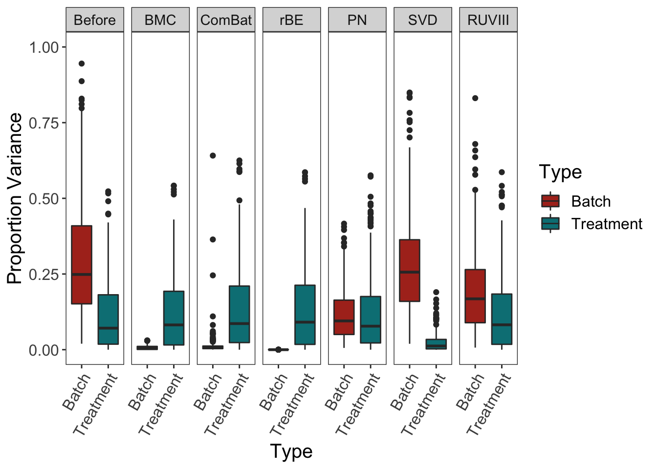
Similar results as in sponge data, BMC, ComBat and removeBatchEffect successfully removed batch variation while preserving treatment variation, but SVD performed poorly. Percentile normalisation and RUVIII preserved sufficient treatment variation, but removed less batch effect variation than BMC, ComBat and removeBatchEffect. It is possible the negative control variables or technical replicate samples did not entirely capture the batch effects. SVD was also inefficient at targeting batch effects, as in AD data the batch effect is present on both first and second components, which results in a miscorrection of batch effects.
4.2.2 RDA
The pRDA method is a multivariate method to assess globally the effect of batch and treatment (two separate models).
# Sponge data
sponge.data.design <- numeric()
sponge.data.design$group <- sponge.trt
sponge.data.design$batch <- sponge.batch

# before
# conditioning on a batch effect
sponge.rda.before1 <- rda(sponge.tss.clr ~ group + Condition(batch),
                         data = sponge.data.design)
sponge.rda.before2 <- rda(sponge.tss.clr ~ batch + Condition(group),
                         data = sponge.data.design)

# amount of variance
sponge.rda.bat_prop.before <- sponge.rda.before1$pCCA$tot.chi*100/sponge.rda.before1$tot.chi
sponge.rda.trt_prop.before <- sponge.rda.before2$pCCA$tot.chi*100/sponge.rda.before2$tot.chi

# BMC
# conditioning on a batch effect
sponge.rda.bmc1 <- rda(sponge.bmc ~ group + Condition(batch),
                      data = sponge.data.design)
sponge.rda.bmc2 <- rda(sponge.bmc ~ batch + Condition(group),
                      data = sponge.data.design)

# amount of variance
sponge.rda.bat_prop.bmc <- sponge.rda.bmc1$pCCA$tot.chi*100/sponge.rda.bmc1$tot.chi
sponge.rda.trt_prop.bmc <- sponge.rda.bmc2$pCCA$tot.chi*100/sponge.rda.bmc2$tot.chi


# combat
# conditioning on a batch effect
sponge.rda.combat1 <- rda(sponge.combat ~ group + Condition(batch),
                         data = sponge.data.design)
sponge.rda.combat2 <- rda(sponge.combat ~ batch + Condition(group),
                         data = sponge.data.design)

# amount of variance
sponge.rda.bat_prop.combat <- sponge.rda.combat1$pCCA$tot.chi*100/sponge.rda.combat1$tot.chi
sponge.rda.trt_prop.combat <- sponge.rda.combat2$pCCA$tot.chi*100/sponge.rda.combat2$tot.chi


# limma
# conditioning on a batch effect
sponge.rda.limma1 <- rda(sponge.limma ~ group + Condition(batch),
                        data = sponge.data.design)
sponge.rda.limma2 <- rda(sponge.limma ~ batch + Condition(group),
                        data = sponge.data.design)

# amount of variance
sponge.rda.bat_prop.limma <- sponge.rda.limma1$pCCA$tot.chi*100/sponge.rda.limma1$tot.chi
sponge.rda.trt_prop.limma <- sponge.rda.limma2$pCCA$tot.chi*100/sponge.rda.limma2$tot.chi


# percentile
# conditioning on a batch effect
sponge.rda.percentile1 <- rda(sponge.percentile ~ group + Condition(batch),
                             data = sponge.data.design)
sponge.rda.percentile2 <- rda(sponge.percentile ~ batch + Condition(group),
                             data = sponge.data.design)

# amount of variance
sponge.rda.bat_prop.percentile <- sponge.rda.percentile1$pCCA$tot.chi*100/sponge.rda.percentile1$tot.chi
sponge.rda.trt_prop.percentile <- sponge.rda.percentile2$pCCA$tot.chi*100/sponge.rda.percentile2$tot.chi


# SVD
# conditioning on a batch effect
sponge.rda.svd1 <- rda(sponge.svd ~ group + Condition(batch),
                      data = sponge.data.design)
sponge.rda.svd2 <- rda(sponge.svd ~ batch + Condition(group),
                      data = sponge.data.design)

# amount of variance
sponge.rda.bat_prop.svd <- sponge.rda.svd1$pCCA$tot.chi*100/sponge.rda.svd1$tot.chi
sponge.rda.trt_prop.svd <- sponge.rda.svd2$pCCA$tot.chi*100/sponge.rda.svd2$tot.chi
We now represent the amount of variance explained by batch and treatment estimated with pRDA:
# proportion
sponge.rda.prop.before <- c(sponge.rda.bat_prop.before,
                           sponge.rda.trt_prop.before)
sponge.rda.prop.bmc <- c(sponge.rda.bat_prop.bmc,
                        sponge.rda.trt_prop.bmc)
sponge.rda.prop.combat <- c(sponge.rda.bat_prop.combat,
                           sponge.rda.trt_prop.combat)
sponge.rda.prop.limma <- c(sponge.rda.bat_prop.limma,
                          sponge.rda.trt_prop.limma)
sponge.rda.prop.percentile <- c(sponge.rda.bat_prop.percentile,
                               sponge.rda.trt_prop.percentile)
sponge.rda.prop.svd <- c(sponge.rda.bat_prop.svd,
                        sponge.rda.trt_prop.svd)

# merge results
sponge.rda.prop.val <- c(sponge.rda.prop.before, sponge.rda.prop.bmc,
                        sponge.rda.prop.combat, sponge.rda.prop.limma,
                        sponge.rda.prop.percentile, sponge.rda.prop.svd)

# add batch, trt and method info
sponge.rda.prop <- data.frame(prop = sponge.rda.prop.val,
                             prop.r = round(sponge.rda.prop.val, 2),
                             Method = rep(c('Before', 'BMC', 'ComBat',
                                            'rBE', 'PN', 'SVD'), each = 2),
                             Type = rep(c('Batch', 'Tissue'), 6))

# reorder levels
sponge.rda.prop$Method <- factor(sponge.rda.prop$Method,
                                levels = unique(sponge.rda.prop$Method))

ggplot(data = sponge.rda.prop, aes(x = Method, y = prop, fill = Type)) +
  geom_bar(stat = "identity", position = 'dodge', colour = 'black') +
  geom_text(data = sponge.rda.prop, aes(Method, prop + 2.5, label = prop.r),
            position = position_dodge(width = 0.9), size = 3) + theme_bw() +
  labs(y = "Variance explained (%)") +
  theme(axis.text.x = element_text(angle = 60, hjust = 1),
        panel.grid = element_blank(), axis.text = element_text(size = 12),
        axis.title = element_text(size = 15), legend.title = element_text(size = 15),
        legend.text = element_text(size = 12)) + ylim(0,100)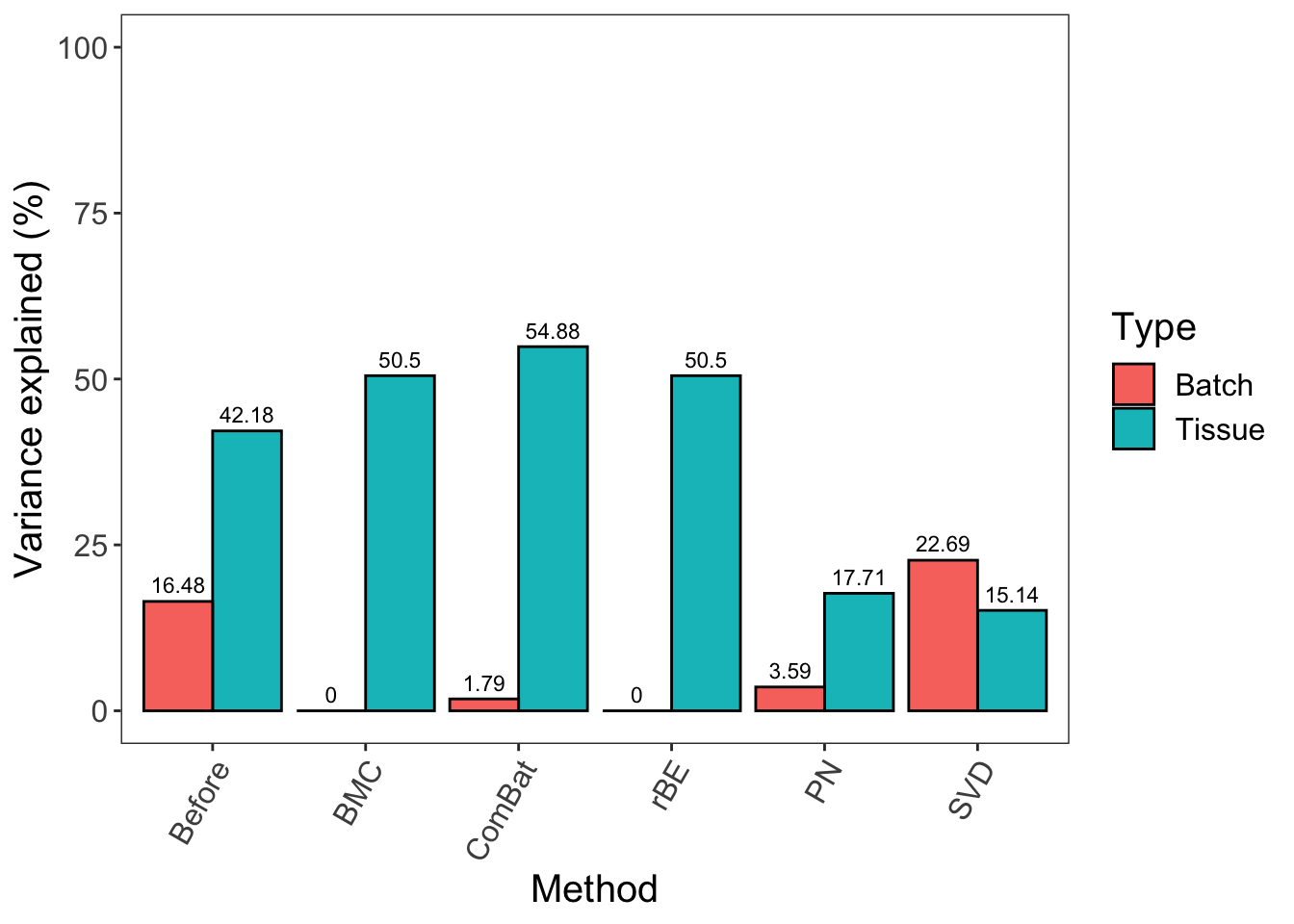
In sponge data, pRDA shows that BMC, ComBat and removeBatchEffect were more efficient at removing batch variation while preserving treatment variation. This result is in agreement with the proportional variance calculated using a linear model in the previous section ‘linear model per variable’. ComBat removed relatively less batch variation compared with the other two methods, which implies that the batch effect is not purely systematic. The low efficiency of percentile normalisation is more obvious in the variance calculated with pRDA. It did not remove enough batch variation, nor preserve enough treatment variation in sponge data.
We also apply pRDA on AD data.
# AD data
ad.data.design <- numeric()
ad.data.design$group <- ad.trt
ad.data.design$batch <- ad.batch

# before
# conditioning on a batch effect
ad.rda.before1 <- rda(ad.clr ~ group + Condition(batch), data = ad.data.design)
ad.rda.before2 <- rda(ad.clr ~ batch + Condition(group), data = ad.data.design)

# amount of variance
ad.rda.bat_prop.before <- ad.rda.before1$pCCA$tot.chi*100/ad.rda.before1$tot.chi
ad.rda.trt_prop.before <- ad.rda.before2$pCCA$tot.chi*100/ad.rda.before2$tot.chi

# BMC
# conditioning on a batch effect
ad.rda.bmc1 <- rda(ad.bmc ~ group + Condition(batch), data = ad.data.design)
ad.rda.bmc2 <- rda(ad.bmc ~ batch + Condition(group), data = ad.data.design)

# amount of variance
ad.rda.bat_prop.bmc <- ad.rda.bmc1$pCCA$tot.chi*100/ad.rda.bmc1$tot.chi
ad.rda.trt_prop.bmc <- ad.rda.bmc2$pCCA$tot.chi*100/ad.rda.bmc2$tot.chi


# combat
# conditioning on a batch effect
ad.rda.combat1 <- rda(ad.combat ~ group + Condition(batch), data = ad.data.design)
ad.rda.combat2 <- rda(ad.combat ~ batch + Condition(group), data = ad.data.design)

# amount of variance
ad.rda.bat_prop.combat <- ad.rda.combat1$pCCA$tot.chi*100/ad.rda.combat1$tot.chi
ad.rda.trt_prop.combat <- ad.rda.combat2$pCCA$tot.chi*100/ad.rda.combat2$tot.chi


# limma
# conditioning on a batch effect
ad.rda.limma1 <- rda(ad.limma ~ group + Condition(batch), data = ad.data.design)
ad.rda.limma2 <- rda(ad.limma ~ batch + Condition(group), data = ad.data.design)

# amount of variance
ad.rda.bat_prop.limma <- ad.rda.limma1$pCCA$tot.chi*100/ad.rda.limma1$tot.chi
ad.rda.trt_prop.limma <- ad.rda.limma2$pCCA$tot.chi*100/ad.rda.limma2$tot.chi


# percentile
# conditioning on a batch effect
ad.rda.percentile1 <- rda(ad.percentile ~ group + Condition(batch),
                         data = ad.data.design)
ad.rda.percentile2 <- rda(ad.percentile ~ batch + Condition(group),
                         data = ad.data.design)

# amount of variance
ad.rda.bat_prop.percentile <- ad.rda.percentile1$pCCA$tot.chi*100/ad.rda.percentile1$tot.chi
ad.rda.trt_prop.percentile <- ad.rda.percentile2$pCCA$tot.chi*100/ad.rda.percentile2$tot.chi


# SVD
# conditioning on a batch effect
ad.rda.svd1 <- rda(ad.svd ~ group + Condition(batch), data = ad.data.design)
ad.rda.svd2 <- rda(ad.svd ~ batch + Condition(group), data = ad.data.design)

# amount of variance
ad.rda.bat_prop.svd <- ad.rda.svd1$pCCA$tot.chi*100/ad.rda.svd1$tot.chi
ad.rda.trt_prop.svd <- ad.rda.svd2$pCCA$tot.chi*100/ad.rda.svd2$tot.chi


# RUVIII
# conditioning on a batch effect
ad.rda.ruv1 <- rda(ad.ruvIII ~ group + Condition(batch), data = ad.data.design)
ad.rda.ruv2 <- rda(ad.ruvIII ~ batch + Condition(group), data = ad.data.design)

# amount of variance
ad.rda.bat_prop.ruv <- ad.rda.ruv1$pCCA$tot.chi*100/ad.rda.ruv1$tot.chi
ad.rda.trt_prop.ruv <- ad.rda.ruv2$pCCA$tot.chi*100/ad.rda.ruv2$tot.chi
# proportion
ad.rda.prop.before <- c(ad.rda.bat_prop.before, ad.rda.trt_prop.before)
ad.rda.prop.bmc <- c(ad.rda.bat_prop.bmc, ad.rda.trt_prop.bmc)
ad.rda.prop.combat <- c(ad.rda.bat_prop.combat, ad.rda.trt_prop.combat)
ad.rda.prop.limma <- c(ad.rda.bat_prop.limma, ad.rda.trt_prop.limma)
ad.rda.prop.percentile <- c(ad.rda.bat_prop.percentile, ad.rda.trt_prop.percentile)
ad.rda.prop.svd <- c(ad.rda.bat_prop.svd, ad.rda.trt_prop.svd)
ad.rda.prop.ruv <- c(ad.rda.bat_prop.ruv, ad.rda.trt_prop.ruv)
# merge results
ad.rda.prop.val <- c(ad.rda.prop.before, ad.rda.prop.bmc,
ad.rda.prop.combat, ad.rda.prop.limma,
ad.rda.prop.percentile, ad.rda.prop.svd,
ad.rda.prop.ruv)
# add batch, trt and method info
ad.rda.prop <- data.frame(prop = ad.rda.prop.val, prop.r = round(ad.rda.prop.val, 2),
Method = rep(c('Before', 'BMC', 'ComBat', 'rBE',
'PN', 'SVD', 'RUVIII'), each = 2),
Type = rep(c('Batch', 'Treatment'), 7))
# reorder levels
ad.rda.prop$Method <- factor(ad.rda.prop$Method, levels = unique(ad.rda.prop$Method))
ggplot(data = ad.rda.prop, aes(x = Method, y = prop, fill = Type)) +
geom_bar(stat = "identity", position = 'dodge', colour = 'black') +
geom_text(data = ad.rda.prop, aes(Method, prop + 2.5, label = prop.r),
position = position_dodge(width = 1), size = 3) + theme_bw() +
labs(y = "Variance explained (%)") +
theme(axis.text.x = element_text(angle = 60, hjust = 1),
panel.grid = element_blank(), axis.text = element_text(size = 12),
axis.title = element_text(size = 15), legend.title = element_text(size = 15),
legend.text = element_text(size = 12)) + scale_fill_hue(l = 40) + ylim(0,100)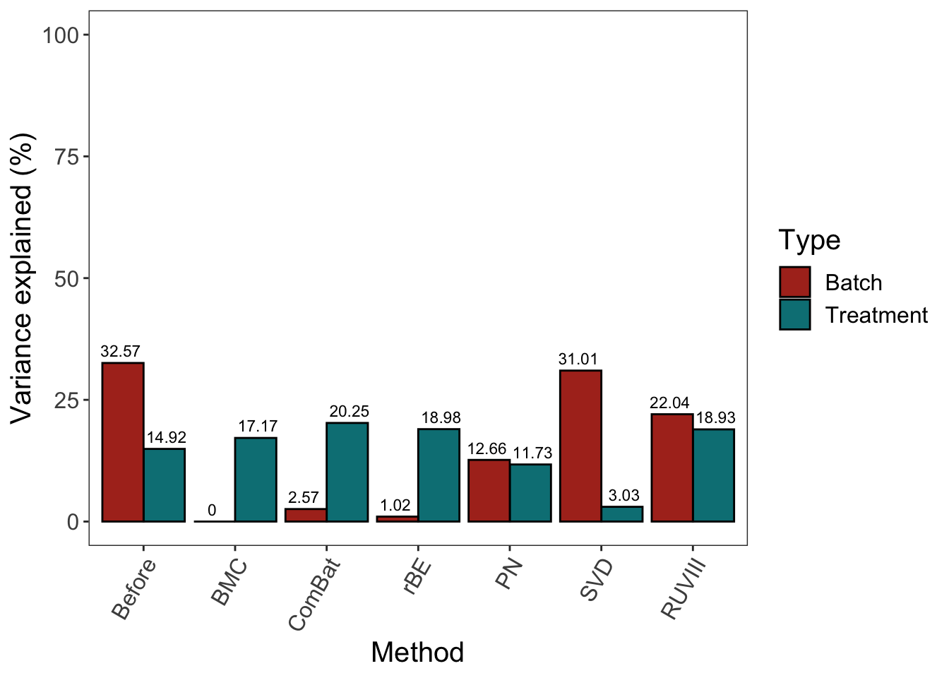
Similar as results from sponge data, BMC, ComBat and removeBatchEffect were more efficient at removing batch variation while preserving treatment variation. ComBat removed relatively less batch variation compared with the other two methods. Percentile normalisation did not remove enough batch variation, nor preserve enough treatment variation in AD data. RUVIII preserved enough treatment variation but did not remove enough batch variation.
In sponge data, the results of BMC and removeBatchEffect are the same, while in AD data, removeBatchEffect removed less batch variation but preserved more treatment variation. This indicates some linear correlation exists between the batch and treatment effects, which might originate from the batch x treatment design.
4.2.3 PVCA
PVCA can be applied as a validation method that complements pRDA, but it requires 42 OTUs minimum. Therefore, it did not apply on sponge data.
# AD data
ad.PVCA.score <- data.frame(Interaction = NA, Batch = NA,
                           Treatment = NA, Residuals = NA)

ad.Bat_Int.factors <- data.frame(Batch = ad.batch, Treatment = ad.trt)
rownames(ad.Bat_Int.factors) <- rownames(ad.clr)
pdata <- AnnotatedDataFrame(ad.Bat_Int.factors)

# before
ad.eset.X.before <- new("ExpressionSet", exprs = t(ad.clr), phenoData = pdata)
ad.pvcaObj.before <- pvcaBatchAssess(ad.eset.X.before, c('Batch', 'Treatment'), 0.6)
ad.values.before <- ad.pvcaObj.before$dat
ad.PVCA.score[1, ] <- ad.values.before

# bmc
ad.eset.X.bmc <- new("ExpressionSet", exprs = t(ad.bmc), phenoData = pdata)
ad.pvcaObj.bmc <- pvcaBatchAssess(ad.eset.X.bmc, c('Batch', 'Treatment'), 0.6)
ad.values.bmc <- ad.pvcaObj.bmc$dat
ad.PVCA.score[2, ] <- ad.values.bmc


# combat

ad.eset.X.combat <- new("ExpressionSet", exprs = t(ad.combat), phenoData = pdata)
ad.pvcaObj.combat <- pvcaBatchAssess(ad.eset.X.combat, c('Batch', 'Treatment'), 0.6)
ad.values.combat <- ad.pvcaObj.combat$dat
ad.PVCA.score[3, ] <- ad.values.combat

# limma

ad.eset.X.limma <- new("ExpressionSet", exprs = t(ad.limma), phenoData = pdata)
ad.pvcaObj.limma <- pvcaBatchAssess(ad.eset.X.limma, c('Batch', 'Treatment'), 0.6)
ad.values.limma <- ad.pvcaObj.limma$dat
ad.PVCA.score[4, ] <- ad.values.limma


# PN

ad.eset.X.percentile <- new("ExpressionSet", exprs = t(ad.percentile),
                            phenoData = pdata)
ad.pvcaObj.percentile <- pvcaBatchAssess(ad.eset.X.percentile,
                                         c('Batch', 'Treatment'), 0.6)
ad.values.percentile <- ad.pvcaObj.percentile$dat
ad.PVCA.score[5, ] <- ad.values.percentile


# svd

ad.eset.X.svd <- new("ExpressionSet", exprs = t(ad.svd), phenoData = pdata)
ad.pvcaObj.svd <- pvcaBatchAssess(ad.eset.X.svd, c('Batch', 'Treatment'), 0.6)
ad.values.svd <- ad.pvcaObj.svd$dat
ad.PVCA.score[6, ] <- ad.values.svd


# RUVIII

ad.eset.X.ruv <- new("ExpressionSet", exprs = t(ad.ruvIII), phenoData = pdata)
ad.pvcaObj.ruv <- pvcaBatchAssess(ad.eset.X.ruv, c('Batch', 'Treatment'), 0.6)
ad.values.ruv <- ad.pvcaObj.ruv$dat
ad.PVCA.score[7, ] <- ad.values.ruv

rownames(ad.PVCA.score) <- c('Before', 'BMC', 'ComBat', 'rBE', 'PN', 'SVD', 'RUVIII')
# merge results
ad.pvca.prop.val <- c(ad.PVCA.score$Batch, ad.PVCA.score$Treatment)
# add batch, trt and method info
ad.pvca.prop <- data.frame(prop = ad.pvca.prop.val, prop.r = round(ad.pvca.prop.val, 2),
Method = rep(c('Before', 'BMC', 'ComBat', 'rBE',
'PN', 'SVD', 'RUVIII'), 2),
Type = rep(c('Batch', 'Treatment'), each = 7))
# reorder levels
ad.pvca.prop$Method <- factor(ad.pvca.prop$Method, levels = unique(ad.pvca.prop$Method))
ggplot(data = ad.pvca.prop, aes(x = Method, y = prop, fill = Type)) +
geom_bar(stat = "identity", position = 'dodge', colour = 'black') +
geom_text(data = ad.pvca.prop, aes(Method, prop + 0.03, label = prop.r),
position = position_dodge(width = 0.9), size = 3) + theme_bw() +
labs(y = "Weighted average proportion variance") +
theme(axis.text.x = element_text(angle = 60, hjust = 1),
panel.grid = element_blank(),axis.text = element_text(size = 12),
axis.title = element_text(size = 15), legend.title = element_text(size = 15),
legend.text = element_text(size = 12)) + scale_fill_hue(l = 40) + ylim(0,1)
Proportionally, BMC, ComBat and removeBatchEffect removed more of the variance explained by batch and maintained more variance explained by treatment than other methods in AD data.
4.2.4 Silhouette coefficient
Finally we assess the quality of the clusters, based on either batch or treatment information using the silhouette coefficient and the PC components. This coefficient measures how cohesive a sample is to its own cluster compared to other clusters. It has been adapted to assess the consistency of sample groups based on treatment or batch effects.
The average silhouette coefficient width across all samples in one group (batch \(\bar{s}_{b}\) or treatment \(\bar{s}_{t}\)) is calculated and plotted here. If \(\bar{s}_{b}\) is close to \(0\) there is no batch effect, and if \(\bar{s}_{t}\) is close to \(1\) or \(-1\) there is a treatment effect.
# Sponge data
sponge.silh.before <- calc.sil(sponge.pca.before$variates$X,
                              y1 = sponge.batch, y2 = sponge.trt,
                              name.y1 = 'Batch', name.y2 = 'Tissue')
sponge.silh.bmc <- calc.sil(sponge.pca.bmc$variates$X,
                           y1 = sponge.batch, y2 = sponge.trt,
                           name.y1 = 'Batch', name.y2 = 'Tissue')
sponge.silh.combat <- calc.sil(sponge.pca.combat$variates$X,
                              y1 = sponge.batch, y2 = sponge.trt,
                              name.y1 = 'Batch', name.y2 = 'Tissue')
sponge.silh.limma <- calc.sil(sponge.pca.limma$variates$X,
                             y1 = sponge.batch, y2 = sponge.trt,
                             name.y1 = 'Batch', name.y2 = 'Tissue')
sponge.silh.percentile <- calc.sil(sponge.pca.percentile$variates$X,
                                  y1 = sponge.batch, y2 = sponge.trt,
                                  name.y1 = 'Batch', name.y2 = 'Tissue')
sponge.silh.svd <- calc.sil(sponge.pca.svd$variates$X,
                           y1 = sponge.batch, y2 = sponge.trt,
                           name.y1 = 'Batch', name.y2 = 'Tissue')


sponge.silh.plot <- rbind(sponge.silh.before, sponge.silh.bmc, sponge.silh.combat,
                         sponge.silh.limma, sponge.silh.percentile, sponge.silh.svd)
sponge.silh.plot$method <- c(rep('Before', nrow(sponge.silh.before)),
                            rep('BMC', nrow(sponge.silh.bmc)),
                            rep('ComBat', nrow(sponge.silh.combat)),
                            rep('rBE', nrow(sponge.silh.limma)),
                            rep('PN', nrow(sponge.silh.percentile)),
                            rep('SVD', nrow(sponge.silh.svd))
)
sponge.silh.plot$method <- factor(sponge.silh.plot$method,
                                 levels = unique(sponge.silh.plot$method))
sponge.silh.plot$Cluster <- factor(sponge.silh.plot$Cluster,
                                   levels = unique(sponge.silh.plot$Cluster))
sponge.silh.plot$Type <- factor(sponge.silh.plot$Type,
                                levels = unique(sponge.silh.plot$Type))


ggplot(sponge.silh.plot, aes(x = Type, y = silh.coeff, color = Cluster, shape = Type)) +
  geom_point() + facet_grid(cols = vars(method)) + theme_bw() +
  theme(axis.text.x = element_text(angle = 60, hjust = 1),
        strip.text = element_text(size = 12), panel.grid = element_blank(),
        axis.text = element_text(size = 12), axis.title = element_text(size = 15),
        legend.title = element_text(size = 15), legend.text = element_text(size = 12)) +
  scale_color_manual(values = c('#388ECC','#F68B33','#F0E442','#D55E00')) +
labs(x = 'Type', y = 'Silhouette Coefficient', name = 'Type') 
\(\bar{s}_{b}\) of different batches in sponge data decreased to \(0\) after correction with BMC, ComBat and removeBatchEffect, while \(\bar{s}_{t}\) of different tissues increased or maintained at the same level as before correction.
We also calculate the silhouette coefficients for AD data.
# AD data
ad.silh.before <- calc.sil(ad.pca.before$variates$X, y1 = ad.batch,
                          y2 = ad.trt, name.y1 = 'Batch', name.y2 = 'Treatment')
ad.silh.bmc <- calc.sil(ad.pca.bmc$variates$X, y1 = ad.batch,
                       y2 = ad.trt, name.y1 = 'Batch', name.y2 = 'Treatment')
ad.silh.combat <- calc.sil(ad.pca.combat$variates$X, y1 = ad.batch,
                          y2 = ad.trt, name.y1 = 'Batch', name.y2 = 'Treatment')
ad.silh.limma <- calc.sil(ad.pca.limma$variates$X, y1 = ad.batch,
                         y2 = ad.trt, name.y1 = 'Batch', name.y2 = 'Treatment')
ad.silh.percentile <- calc.sil(ad.pca.percentile$variates$X, y1 = ad.batch,
                              y2 = ad.trt, name.y1 = 'Batch', name.y2 = 'Treatment')
ad.silh.svd <- calc.sil(ad.pca.svd$variates$X, y1 = ad.batch,
                       y2 = ad.trt, name.y1 = 'Batch', name.y2 = 'Treatment')
ad.silh.ruv <- calc.sil(ad.pca.ruv$variates$X, y1 = ad.batch,
                       y2 = ad.trt, name.y1 = 'Batch', name.y2 = 'Treatment')


ad.silh.plot <- rbind(ad.silh.before, ad.silh.bmc, ad.silh.combat,
                     ad.silh.limma, ad.silh.percentile, ad.silh.svd, ad.silh.ruv)
ad.silh.plot$method <- c(rep('Before', nrow(ad.silh.before)),
                        rep('BMC', nrow(ad.silh.bmc)),
                        rep('ComBat', nrow(ad.silh.combat)),
                        rep('rBE', nrow(ad.silh.limma)),
                        rep('PN', nrow(ad.silh.percentile)),
                        rep('SVD', nrow(ad.silh.svd)),
                        rep('RUVIII', nrow(ad.silh.ruv))
)
ad.silh.plot$method <- factor(ad.silh.plot$method, levels = unique(ad.silh.plot$method))
ad.silh.plot$Cluster <- factor(ad.silh.plot$Cluster, levels = unique(ad.silh.plot$Cluster))
ad.silh.plot$Type <- factor(ad.silh.plot$Type, levels = unique(ad.silh.plot$Type))

ggplot(ad.silh.plot, aes(x = Type, y = silh.coeff, color = Cluster, shape = Type)) +
  geom_point() + facet_grid(cols = vars(method)) + theme_bw() +
  theme(axis.text.x = element_text(angle = 60, hjust = 1),
        strip.text = element_text(size = 12), panel.grid = element_blank(),
        axis.text = element_text(size = 10), axis.title = element_text(size = 15),
        legend.title = element_text(size = 15), legend.text = element_text(size = 12)) +
  scale_color_manual(values = c('#388ECC', '#F68B33', '#C2C2C2', '#009E73',
                                '#CC79A7', '#0072B2', '#999999')) +
labs(x = 'Type', y = 'Silhouette Coefficient', name = 'Type') 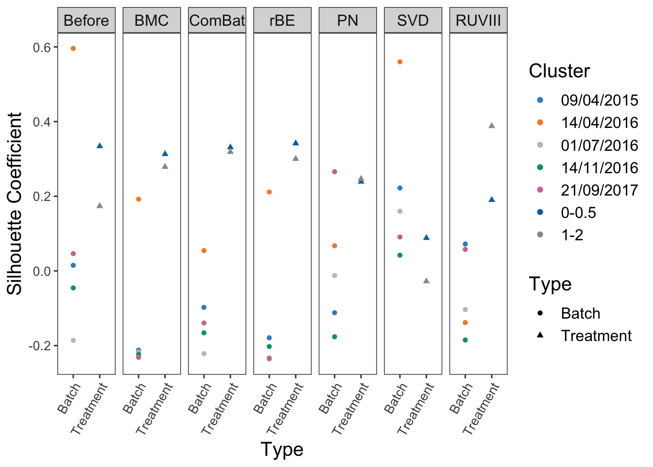
In AD data that includes five batches, the interpretation of the results is challenging. After correction, BMC, ComBat, removeBatchEffect, percentile normalisation and RUVIII decreased the batch silhouette coefficients for the batch dated 14/04/2016, but increased the coefficients for the other batches. Therefore it is difficult to assess the efficiency of these methods in this particular case.